2011 EMC Directory & Design Guide - Interference Technology

standards
O n t h e N at ur e a nd Us e of t h e 1.04 m El e c t ric Fiel d Probe
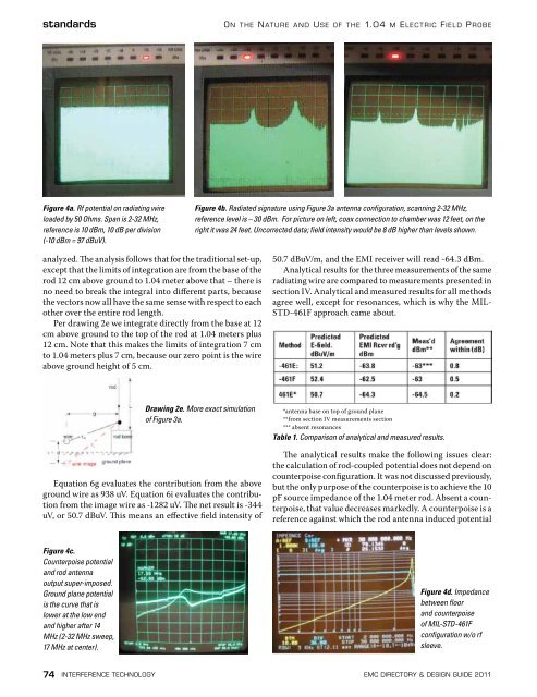
Figure 4a. Rf potential on radiating wire
loaded by 50 Ohms. Span is 2-32 MHz,
reference is 10 dBm, 10 dB per division
(-10 dBm = 97 dBuV).
Figure 4b. Radiated signature using Figure 3a antenna configuration, scanning 2-32 MHz,
reference level is – 30 dBm. For picture on left, coax connection to chamber was 12 feet, on the
right it was 24 feet. Uncorrected data; field intensity would be 8 dB higher than levels shown.
analyzed. The analysis follows that for the traditional set-up,
except that the limits of integration are from the base of the
rod 12 cm above ground to 1.04 meter above that – there is
no need to break the integral into different parts, because
the vectors now all have the same sense with respect to each
other over the entire rod length.
Per drawing 2e we integrate directly from the base at 12
cm above ground to the top of the rod at 1.04 meters plus
12 cm. Note that this makes the limits of integration 7 cm
to 1.04 meters plus 7 cm, because our zero point is the wire
above ground height of 5 cm.
50.7 dBuV/m, and the EMI receiver will read -64.3 dBm.
Analytical results for the three measurements of the same
radiating wire are compared to measurements presented in
section IV. Analytical and measured results for all methods
agree well, except for resonances, which is why the MIL-
STD-461F approach came about.
Drawing 2e. More exact simulation
of Figure 3a.
Equation 6g evaluates the contribution from the above
ground wire as 938 uV. Equation 6i evaluates the contribution
from the image wire as -1282 uV. The net result is -344
uV, or 50.7 dBuV. This means an effective field intensity of
*antenna base on top of ground plane
**from section IV measurements section
*** absent resonances
Table 1. Comparison of analytical and measured results.
The analytical results make the following issues clear:
the calculation of rod-coupled potential does not depend on
counterpoise configuration. It was not discussed previously,
but the only purpose of the counterpoise is to achieve the 10
pF source impedance of the 1.04 meter rod. Absent a counterpoise,
that value decreases markedly. A counterpoise is a
reference against which the rod antenna induced potential
Figure 4c.
Counterpoise potential
and rod antenna
output super-imposed.
Ground plane potential
is the curve that is
lower at the low end
and higher after 14
MHz (2-32 MHz sweep,
17 MHz at center).
Figure 4d. Impedance
between floor
and counterpoise
of MIL-STD-461F
configuration w/o rf
sleeve.
74 interference technology emc Directory & design guide 2011