DARPA ULTRALOG Final Report - Industrial and Manufacturing ...

4
t Si
t
∫ + ( )
i )
t
When RA i (t) remains constant S i (t) becomes:
RA ( τ dτ
= P . (4)
i
Pi
Si ( t)
= . (5)
RA ( t)
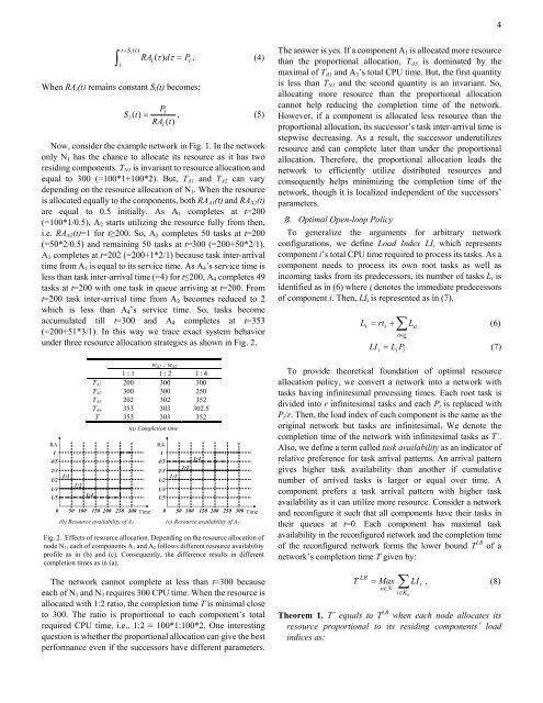
Now, consider the example network in Fig. 1. In the network
only N 1 has the chance to allocate its resource as it has two
residing components. T N1 is invariant to resource allocation and
equal to 300 (=100*1+100*2). But, T A1 and T A2 can vary
depending on the resource allocation of N 1 . When the resource
is allocated equally to the components, both RA A1 (t) and RA A2 (t)
are equal to 0.5 initially. As A 1 completes at t=200
(=100*1/0.5), A 2 starts utilizing the resource fully from then,
i.e. RA A2 (t)=1 for t≥200. So, A 2 completes 50 tasks at t=200
(=50*2/0.5) and remaining 50 tasks at t=300 (=200+50*2/1).
A 3 completes at t=202 (=200+1*2/1) because task inter-arrival
time from A 1 is equal to its service time. As A 4 ’s service time is
less than task inter-arrival time (=4) for t≤200, A 4 completes 49
tasks at t=200 with one task in queue arriving at t=200. From
t=200 task inter-arrival time from A 2 becomes reduced to 2
which is less than A 4 ’s service time. So, tasks become
accumulated till t=300 and A 4 completes at t=353
(=200+51*3/1). In this way we trace exact system behavior
under three resource allocation strategies as shown in Fig. 2.
RA
1
4/5
2/3
1/2
1/3
1/5
1:1
1:2
1:4
0 50 100 150 200 250
w A1 : w A2
1 : 1 1 : 2 1 : 4
T A1 200 300 300
T A2 300 300 250
T A3 202 302 352
T A4 353 303 302.5
T 353 303 352
(a) Completion time
300 Time
The network cannot complete at less than t=300 because
each of N 1 and N 3 requires 300 CPU time. When the resource is
allocated with 1:2 ratio, the completion time T is minimal close
to 300. The ratio is proportional to each component’s total
required CPU time, i.e., 1:2 ≡ 100*1:100*2. One interesting
question is whether the proportional allocation can give the best
performance even if the successors have different parameters.
i
RA
1
1/2
1/3
1/5
0 50 100 150 200 250 300 Time
(b) Resource availability of A 1 (c) Resource availability of A 2
Fig. 2. Effects of resource allocation. Depending on the resource allocation of
node N 1 , each of components A 1 and A 2 follows different resource availability
profile as in (b) and (c). Consequently, the difference results in different
completion times as in (a).
4/5
2/3
1:1
1:2
1:4
The answer is yes. If a component A 1 is allocated more resource
than the proportional allocation, T A3 is dominated by the
maximal of T A1 and A 3 ’s total CPU time. But, the first quantity
is less than T N1 and the second quantity is an invariant. So,
allocating more resource than the proportional allocation
cannot help reducing the completion time of the network.
However, if a component is allocated less resource than the
proportional allocation, its successor’s task inter-arrival time is
stepwise decreasing. As a result, the successor underutilizes
resource and can complete later than under the proportional
allocation. Therefore, the proportional allocation leads the
network to efficiently utilize distributed resources and
consequently helps minimizing the completion time of the
network, though it is localized independent of the successors’
parameters.
B. Optimal Open-loop Policy
To generalize the arguments for arbitrary network
configurations, we define Load Index LI i which represents
component i’s total CPU time required to process its tasks. As a
component needs to process its own root tasks as well as
incoming tasks from its predecessors, its number of tasks L i is
identified as in (6) where i denotes the immediate predecessors
of component i. Then, LI i is represented as in (7).
∑
L = rt + L
(6)
i
i
i
a∈i
LI = L P
To provide theoretical foundation of optimal resource
allocation policy, we convert a network into a network with
tasks having infinitesimal processing times. Each root task is
divided into r infinitesimal tasks and each P i is replaced with
P i /r. Then, the load index of each component is the same as the
original network but tasks are infinitesimal. We denote the
completion time of the network with infinitesimal tasks as T´.
Also, we define a term called task availability as an indicator of
relative preference for task arrival patterns. An arrival pattern
gives higher task availability than another if cumulative
number of arrived tasks is larger or equal over time. A
component prefers a task arrival pattern with higher task
availability as it can utilize more resource. Consider a network
and reconfigure it such that all components have their tasks in
their queues at t=0. Each component has maximal task
availability in the reconfigured network and the completion time
of the reconfigured network forms the lower bound T LB of a
network’s completion time T given by:
T
LB
= Max
n∈N
i
i
∑
i∈
K n
a
LI
i
(7)
. (8)
Theorem 1. T´ equals to T LB when each node allocates its
resource proportional to its residing components’ load
indices as: