DARPA ULTRALOG Final Report - Industrial and Manufacturing ...

More documents

Recommendations

Info

In the rest of this paper we report a queuing model that is useful in supply chain analysis. We explain our rationale for selecting this model for adaptation to the logistics domain. For some of the other models existing in literature, refer to [6][7]. We extend the queuing model and apply it to the logistics scenario in the Cougaar architecture and discuss the results. We raise the fundamental question of how we can use these results for further analysis and control of a logistics system. 3 SUPPLY CHAIN AND NONLINEARITY The notion of evolution over time falls into the realm of what physicists call dynamics. Logistics systems are dynamic. Their behavior can be nonlinear. Therefore we can model a logistics system using the principles of nonlinear dynamics. A supply chain is an example of a logistics system. A typical supply chain exhibits stable behavior with damped oscillations in response to external disturbances. Unstable phenomena however can arise, due to feedback structure, inherent adjustment delays [6], nonlinear decision-making [7] and interactions that go in a supply chain. One of the causes of unstable phenomena is that the information feedback in the system is slow relative to rate of changes that occur in the system. Nonlinearity is inherent in a supply chain. The first mode of unstable behavior to arise in nonlinear systems is usually the simple one-cycle self-sustained oscillations. If the instability drives the system further into the nonlinear regime, more complicated temporal behavior may be generated. The route to chaos through subsequent period-doubling bifurcations, as certain parameters of the system are varied, is generic to large class of systems in physics, chemistry, biology, economics and other fields. Functioning in chaotic regime deprives us the ability for long-term predictions about the behavior of the system, while short-term predictions may be possible sometimes. As a result, control and stabilization of such a system becomes almost impossible. Here we investigate such dynamical behaviors that can arise in models that represent some of the components in a supply chain. 3.1 Preemptive Queuing Model with Delays The Queuing system [8] considered here has two queues (A and B) and a single server with following characteristics: •Once served, the class A customer returns as a class B customer after a constant interval of time •Class B has non-preemptive priority over class A, i.e., the class A queue does not get served until the class B queue is emptied. •Schedules are organized every T units of time, i.e., if the low priority queue is emptied within time T, the server remains idle for the remaining time interval. •Finally, the higher priority class B has a lower service rate than the low priority class A Suppose the system is sampled at the end of every schedule cycle, and the following quantities are observed at the beginning of the kth interval: Ak the queue length of low priority queue, Bk the queue length of high priority queue, C k the outflow from low priority queue in the kth interval and Dk the outflow from high priority queue in the kth interval. In the model, λ k denotes the arrival rate, µ a is the service rate for the lower priority queue, µ b is the service rate for the higher priority queue and l the feedback interval in units of the schedule cycle. The following four equations then completely describe the evolution of the system: Ak + 1 = Ak + λk − Ck (3) C B k min( A k Dk + λk , µ a (1 − )) µ = (4) k +1 = Bk + Ck −l − Dk (5) D min( B + C , µ ) k = k k −l b (6) Equations (3) and (5) are merely conservation rules, while equations (4) and (6) model the constraints on the outflows and the interaction between the queues. This model while conceptually simple, exhibits surprisingly complex behaviors. The dynamical behavior reported in [8] is summarized in the following. Figure 1: Non-preemptive Queuing Model Dynamical Behavior: The analytic approach to solve for the flow model under constant arrivals (i.e. b λ = k λ for all k) shows several classes of solutions. The system is found to batch its workload even for such perfectly smooth arrival patterns. Following are the characteristics of behavior of the system: •Above a threshold arrival rate ( λ ≥ µ b / 2 ), a momentary overload can send the system into a number of stable modes of oscillations. •Each mode of oscillations is characterized by distinct average queuing delays. •Extreme sensitivity to parameters, and the existence of chaos, implies that the system at a given time may be in any one of a number of distinct steady-state modes. The batching of the workload can cause significant queuing delays even at moderate occupancies. Also such oscillatory behavior significantly lowers the real-time capacity of the system. 4 APPLICATION OF QUEUING MODEL TO LOGISTICS SCENARIO The assumptions in the model proposed by [8] are generic in the sense that priorities are widely observed in large systems due to economic and administrative compulsions. Sometime they can also arise from the physical facts when two different stages of processing have certain temporal constraint. Priorities may also arise due to the nonhomogeneity of the system where “knowledge” level of one agent is different from the other. Varying service time again follows from physical constraints on the task. For example in a simple logistics scenario tasks like unpacking, shipping, logging and dispatching may take different times. These times scales can vary widely depending on the nature and physical characteristics of the tasks. The considerations regarding the generality of assumptions and the clear one-to-one correspondence
etween the physical logistics tasks and the model parameters described in [8] made us apply the queuing model to a simple, yet, realistic logistics scenario. 4.1 Example Logistics Scenario The example scenario consists of two stages modeled by the non-preemptive queuing formalism. We take a simple battle front scenario (this can be any context of supply of materials, not necessarily battle front). During the first stage, supplies are processed by the node (agent) This involves two tasks: Unpacking (Task A) and Shipping (Task B). Our assumptions are that shipping takes more resources than packing, shipping gets a non preemptive priority and resources are common to both the tasks The second stage consists of disbursement of supplies. The output of first stage feeds into the second stage (as arrival). The two associated tasks are: Maintaining an inventory (Task A) and Disbursing the supply to the troops (Task B). The assumptions at stage two are that disbursing takes more resources than maintaining inventory, disbursing has a non pre-emptive priority and resources are common to both the tasks. Figure 1 shows the queuing model. This is figure is reproduced from [8]. It must be noted that that rules are very simple and generic. Priority and heterogeneity are fundamental to any logistic planning and scheduling. Tasks have to be prioritized in order to do the most important thing first. This comes naturally as we try to optimize an objective and assign the tasks their "importance.” In addition in all logistics systems, resources are limited, both in time and space. Temporal constraints considered in the example are realistic, in the sense that you cannot disburse supplies without unpacking them. Temporal dependence plays an important role in logistic planning (interdependency). This simple example also simulates the effect of arbitrary but bounded initial conditions Cougaar (Cognitive Agent Architecture) is developed under DARPA Advanced Logistics Program (ALP). Survivability of Cougaar is addressed in the UltraLog program of DARPA. In the above example each stage is modeled as an agent. The activities are modeled as agent processes. We do not discuss Cougaar architecture in this paper. Details can be found at the URL: http://www.couggar.org. 4.2 Analysis One of the hallmarks of chaos is sensitive dependency to initial conditions (SDIC). External environment (the world in which the logistics scenario resides) changes and hence changing the initial conditions and the parameters. The following affects the initial conditions and parameters of the agents ( thereby affecting the initial conditions of the queuing model): change in arrival rate of supplies (inputs to the agents), change in resources (assets) available in each agent, and delay in processing of Tasks. The internal states of the two agents are characterized by: supplies waiting to be shipped (X 1 ), supplies waiting to be unpacked (X 2 ), supplies actually shipped, supplies waiting to be inventoried (X 3 ), supplies waiting to be disbursed (X 4 ) to the troops and supplies actually shipped. We have considered these variables and observed their behavior. Characterization of these behaviors leads to some interesting inferences. We simulated the queuing models in each agent with the following model parameters. There are 162 personnel in each of the agents, who can be allocated to either task. We assume that it takes 1 unit of time and one person to do task A and one unit of time with 2 people to do task B. This defines the capacity/arrival rate as 54 items/unit time. Hence arrival rate can be 0-54 per unit time. 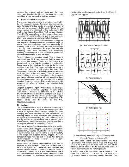We assume that the initial conditions are given by: X10=131, X20=201, X30=151 and X40=29. S tate X 1andX2-> M agnitude(dB) P o w er S pectru m 120 100 80 60 40 20 50 40 30 20 10 0 -10 -20 -30 Evolution of system states 50 55 60 65 70 75 80 85 90 95 100 Time-> (a): Time evolution of system state Power Spectrum of state X1 -40 0 0.1 0.2 0.3 0.4 0.5 0.6 0.7 0.8 0.9 1 Frequency 50 (b) Power spectrum State space trajectories for center 2(blue) and for center 1(red) 150 100 2 ,x4-> x 0 0 50 100 150 x1,x3-> (c) State-space plot d) Multi-stability:Bifurcation diagram for the system Figure 2: Plots for arrival rate =53 We have used Matlab for computations. We have experimented with several arrival rates and delays. We observe the state-space structure (time evolution) of the following: arrival rates at all the queues, time series of various parameters and the Power-spectrum. At arrival rates of 40 the system has a period of 1, at arrival rate of 50 a period 2, at 52 a period of 4 and at 53 the system shows a seemingly random behavior. This
Page 1 and 2:
Ultra*Log PSU/IAI Final Report for
Page 3 and 4:
Contents Contents .................
Page 5:
Executive Summary Ultra*Log is a De
Page 8 and 9:
2.3 Gnanasambandam, N., Lee, S., Ku
Page 10 and 11:
6 Characterization and analysis of
Page 12 and 13:
timizing simultaneously the link de
Page 14 and 15:
where ∆ 1 (j) ≥ 0 and ∆ 2 (i,
Page 16 and 17:
Table 2. GA Results Agent N A D max
Page 18 and 19:
connected component, in which a pat
Page 20 and 21:
Random Small-world Scale-free with
Page 22 and 23:
Growth mechanisms Start with a smal
Page 24 and 25:
Table 2. The proposed network’s c
Page 26 and 27:
¡ ¡ ¢ £ ¤ ¥ ¦ £ § ¨ © ¥
Page 28 and 29:
© © ¤ ¢ ¨ ¤ £ ¦ ¨ © §
Page 30 and 31:
DMAS Controller. The functional uni
Page 32 and 33:
1000 500 0 -500 -1000 0.2 0.4 0.6 0
Page 34 and 35:
tems. Proceedings of the Second Joi
Page 36 and 37:
Proceedings of the 1st Open Cougaar
Page 38 and 39:
Page 40 and 41:
Page 42 and 43:
Page 44 and 45:
1 SITUATION IDENTIFICATION USING DY
Page 46 and 47:
3 3.2 Behavior In SSC society an ag
Page 48 and 49:
5 All the behavior parameters may n
Page 50 and 51:
Estimating Global Stress Environmen
Page 52 and 53:
chaotic deterministic time series.
Page 54 and 55:
100% 1 95% 2 14 15 64% TAO 4 64% 62
Page 56 and 57:
interactions as a dynamical system
Page 58 and 59:
ehavior states under varying system
Page 60 and 61:
Extensive testing and validation of
Page 62 and 63:
5 Conclusions and Future Research T
Page 64 and 65:
2 to function critically even under
Page 66 and 67:
4 points into a corresponding inner
Page 68 and 69:
6 stresses well. The Warehouse 1 ag
Page 70 and 71:
© £ ¨ ¥ ¤ § ¢ ¥ ©
Page 72 and 73:
Table 1: Notation Symbol Descriptio
Page 74 and 75:
4 Conclusions and Future Work 4.1 C
Page 76 and 77:
O, U Stresses Physical/Infrastructu
Page 78 and 79:
Manuscript for IEEE Transactions on
Page 80 and 81:
Page 82 and 83:
Page 84 and 85:
Page 86 and 87:
Page 88 and 89:
Page 90 and 91:
Page 92 and 93:
Page 94 and 95:
Page 96 and 97:
Page 98 and 99:
Page 100 and 101:
Page 102 and 103:
Page 104 and 105:
Page 106 and 107:
2 discuss problem domain and in Sec
Page 108 and 109:
4 t Si t ∫ + ( ) i ) t When RA i
Page 110 and 111:
6 S UB i ∑ = P LI / LI . (16) i p
Page 112 and 113:
8 policies while underutilizing in
Page 114 and 115:
architecture based on both the Grid
Page 116 and 117:
to machines (network topology) and
Page 118 and 119:
component is a member of one of the
Page 120 and 121:
denotes the immediate predecessors
Page 122 and 123:
limit of large number of tasks. If
Page 124 and 125:
Min-min heuristic algorithm Step 1:
Page 126 and 127:
We set up eight different experimen
Page 128 and 129:
0. 4 8057 8237 0.5 6439 6635 0.6 53
Page 130 and 131:
pp. 191-200. [3] I. Foster, C. Kess
Page 132 and 133:
Technology, Cambridge, MA, 1995. [2
Page 134 and 135:
Manuscript for IEEE TRANSACTIONS ON
Page 136 and 137:
Page 138 and 139:
Page 140 and 141:
Page 142 and 143:
Page 144 and 145:
Page 146 and 147:
Page 148 and 149:
Page 150 and 151:
Page 152 and 153:
Page 154 and 155: Manuscript for IEEE TRANSACTIONS ON
Page 156 and 157: Coordinating Control Decisions of S
Page 158 and 159: directly. It has coarser scale. It
Page 160 and 161: Understanding Agent Societies Using
Page 162 and 163: • For tasks, the UID of the direc
Page 164 and 165: for tracking the dependencies betwe
Page 166 and 167: within the monitored enclave. With
Page 168 and 169: Figure 1. Agent Hierarchy in CPE So
Page 170 and 171: Figure 3. The World Model CPY Agent
Page 172 and 173: Table 2. TechSpecs: Infrastructure
Page 174 and 175: terms of the average waiting times
Page 176 and 177: Acknowledgements The work described
Page 178 and 179: key realization to tackle this prob
Page 180 and 181: are or ignored perturbations. The e
Page 182 and 183: sustained oscillations. If the inst
Page 184 and 185: solved by biological systems for li
Page 186 and 187: non-linear and non-stationarity. Ne
Page 188 and 189: D k : Outflow from high priority qu
Page 190 and 191: the system starts to perform self-s
Page 192 and 193: sustained in a supply chain. Resour
Page 194 and 195: which are necessary to make good mo
Page 196 and 197: focusing on the computational compl
Page 198 and 199: line of research that deals with ne
Page 200 and 201: ealizable. But the inherent complex
Page 202 and 203: Min, H. and Zhou, G., 2002, Supply
Page 206: shows relatively irregular behavior
show all

DARPA ULTRALOG Final Report - Industrial and Manufacturing ...

You also want an ePaper? Increase the reach of your titles

Delete template?

Save as template?