DARPA ULTRALOG Final Report - Industrial and Manufacturing ...

6
S
UB
i
∑
= P LI / LI . (16)
i
p∈K
n(
i)
So, a component i can complete by T LB and generate tasks at
a constant interval of T LB /L i from t=S i UB when it receives
tasks at a constant interval of T LB /L i from t=0. Now, consider
component i’s successor s which has only one predecessor.
As the successor receives tasks at a constant interval of T LB /L s
from t=S i UB or more preferably, it can complete by S i UB +T LB .
So, a component e∈E (with no successor) can receive tasks at
a constant interval of T LB /L e from maximal task traveling time
to the component of:
Max
j∈S
e
∑
i∈
j
S
p
UB
i
i
(17)
(note that a path j does not include component e) or more
preferably so that its completion time T e is bounded as:
T
e
≤ T
LB
+ Max
j∈S
e
∑
i∈
j
S
UB
i
. (18)
And, the upper bound of T is the maximal of the bounds.
Though we formulated the upper bound performance
without considering stress environments, one can easily modify
it so that the upper bound performance can reflect the stress
environments (if each ω n s is identifiable or assumable). The
adequacy criterion is defined as the ratio between T LB and T UB
as in (19). When the criterion is close to one, a network can
achieve the lower bound performance using the proportion
allocation policy. Typically, the criterion converges to one as
each L i increases. However, as the criterion approaches zero,
the policy become more and more inadequate. The example
network in Fig. 1 is quite adequate because the network’s
adequacy is 0.99 (300/303).
LB
T
Adequacy = (19)
UB
T
So far, we assumed a hypothetical weighted round-robin
server which is difficult to realize in practice. But, our
arguments do not seem to be invalid because they are based on
worst-case analysis and quantum size is relatively infinitesimal
compared to working horizon in reality.
D. Resource control mechanism
Once a network has an appropriate adequacy over a certain
level (depending on the nature of the network), the proportional
allocation is deployed periodically under MPC framework.
Consider current time as t. To update load index as the system
moves on, we slightly modify it to represent total CPU time for
the remaining tasks as:
LI ( t ) = R ( t ) + L ( t ) P , (20)
i
i
in which R i (t) denotes remaining CPU time for a task in process
and L i (t) the number of remaining tasks excluding a task in
process. After identifying initial number of tasks L i (0)=L i , each
component updates it by counting down as they process tasks.
Periodically, a resource manager of each node collects current
LI i (t)s from residing components and allocates resource
proportional to the indices as in (21). As the resource allocation
policy is purely localized there is no need for synchronization
between nodes. The designed resource control mechanism is
scalable as each node can make decisions independent of
others while requiring almost no computation.
w
i
i ( t)
ωn(
i)
∑ LI p ( t)
p∈K
n(
i)
i
i
LI ( t)
= (21)
VI. EMPIRICAL RESULTS
We ran several experiments using discrete-event simulation
to validate the designed resource control mechanism.
A. Experimental design
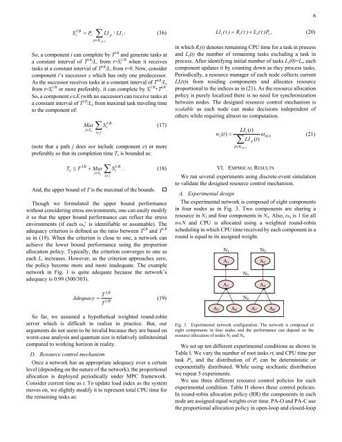
The experimental network is composed of eight components
in four nodes as in Fig. 3. Two components are sharing a
resource in N 3 and four components in N 4 . Also, ω n is 1 for all
n∈N and CPU is allocated using a weighted round-robin
scheduling in which CPU time received by each component in a
round is equal to its assigned weight.
N 1 N 2
A 1
N 3
A 3 A 4
N 4
A 5 A 6 A 7 A 8
Fig. 3. Experimental network configuration. The network is composed of
eight components in four nodes and the performance can depend on the
resource allocation of nodes N 3 and N 4 .
We set up ten different experimental conditions as shown in
Table I. We vary the number of root tasks rt i and CPU time per
task P i , and the distribution of P i can be deterministic or
exponentially distributed. While using stochastic distribution
we repeat 5 experiments.
We use three different resource control policies for each
experimental condition. Table II shows these control policies.
In round-robin allocation policy (RR) the components in each
node are assigned equal weights over time. PA-O and PA-C use
the proportional allocation policy in open-loop and closed-loop
A 2