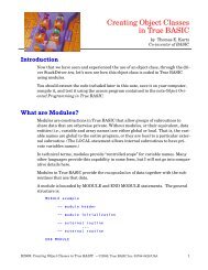
Download the documentation - True BASIC

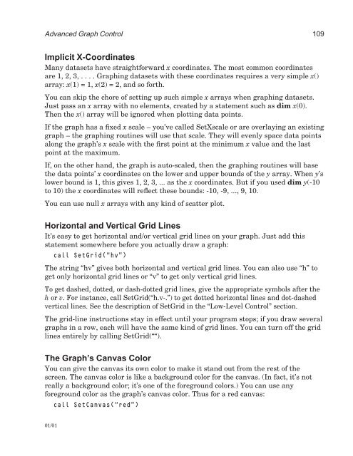
Advanced Graph Control 109
Implicit X-Coordinates
Many datasets have straightforward x coordinates. The most common coordinates
are 1, 2, 3, . . . . Graphing datasets with these coordinates requires a very simple x()
array: x(1) = 1, x(2) = 2, and so forth.
You can skip the chore of setting up such simple x arrays when graphing datasets.
Just pass an x array with no elements, created by a statement such as dim x(0).
Then the x() array will be ignored when plotting data points.
If the graph has a fixed x scale – you’ve called SetXscale or are overlaying an existing
graph – the graphing routines will use that scale. They will evenly space data points
along the graph’s x scale with the first point at the minimum x value and the last
point at the maximum.
If, on the other hand, the graph is auto-scaled, then the graphing routines will base
the data points’ x coordinates on the lower and upper bounds of the y array. When y’s
lower bound is 1, this gives 1, 2, 3, ... as the x coordinates. But if you used dim y(-10
to 10) the x coordinates will reflect these bounds: -10, -9, ..., 9, 10.
You can use null x arrays with any kind of scatter plot.
Horizontal and Vertical Grid Lines
It’s easy to get horizontal and/or vertical grid lines on your graph. Just add this
statement somewhere before you actually draw a graph:
call SetGrid(“hv”)
The string “hv” gives both horizontal and vertical grid lines. You can also use “h” to
get only horizontal grid lines or “v” to get only vertical grid lines.
To get dashed, dotted, or dash-dotted grid lines, give the appropriate symbols after the
h or v. For instance, call SetGrid(“h.v-.”) to get dotted horizontal lines and dot-dashed
vertical lines. See the description of SetGrid in the “Low-Level Control” section.
The grid-line instructions stay in effect until your program stops; if you draw several
graphs in a row, each will have the same kind of grid lines. You can turn off the grid
lines entirely by calling SetGrid(““).
The Graph’s Canvas Color
You can give the canvas its own color to make it stand out from the rest of the
screen. The canvas color is like a background color for the canvas. (In fact, it’s not
really a background color; it’s one of the foreground colors.) You can use any
foreground color as the graph’s canvas color. Thus for a red canvas:
call SetCanvas(“red”)
01/01