Master Thesis - Fachbereich Informatik

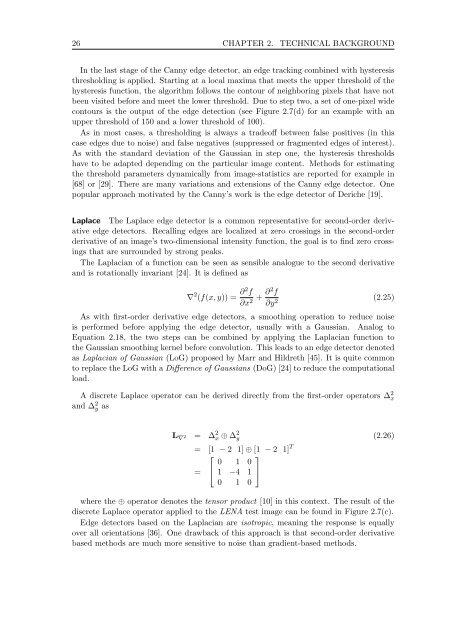
26 CHAPTER 2. TECHNICAL BACKGROUND
In the last stage of the Canny edge detector, an edge tracking combined with hysteresis
thresholding is applied. Starting at a local maxima that meets the upper threshold of the
hysteresis function, the algorithm follows the contour of neighboring pixels that have not
been visited before and meet the lower threshold. Due to step two, a set of one-pixel wide
contours is the output of the edge detection (see Figure 2.7(d) for an example with an
upper threshold of 150 and a lower threshold of 100).
As in most cases, a thresholding is always a tradeoff between false positives (in this
case edges due to noise) and false negatives (suppressed or fragmented edges of interest).
As with the standard deviation of the Gaussian in step one, the hysteresis thresholds
have to be adapted depending on the particular image content. Methods for estimating
the threshold parameters dynamically from image-statistics are reported for example in
[68] or [29]. There are many variations and extensions of the Canny edge detector. One
popular approach motivated by the Canny’s work is the edge detector of Deriche [19].
Laplace The Laplace edge detector is a common representative for second-order derivative
edge detectors. Recalling edges are localized at zero crossings in the second-order
derivative of an image’s two-dimensional intensity function, the goal is to find zero crossings
that are surrounded by strong peaks.
The Laplacian of a function can be seen as sensible analogue to the second derivative
and is rotationally invariant [24]. It is defined as
∇ 2 (f(x, y)) = ∂2 f
∂x 2 + ∂2 f
∂y 2
(2.25)
As with first-order derivative edge detectors, a smoothing operation to reduce noise
is performed before applying the edge detector, usually with a Gaussian. Analog to
Equation 2.18, the two steps can be combined by applying the Laplacian function to
the Gaussian smoothing kernel before convolution. This leads to an edge detector denoted
as Laplacian of Gaussian (LoG) proposed by Marr and Hildreth [45]. It is quite common
to replace the LoG with a Difference of Gaussians (DoG) [24] to reduce the computational
load.
A discrete Laplace operator can be derived directly from the first-order operators ∆ 2 x
and ∆ 2 y as
L∇2 = ∆ 2 x ⊕ ∆ 2 y (2.26)
= [1 − 2 1]⊕ [1 − 2 1] T
⎡
⎤
0 1 0
= ⎣ 1 −4 1 ⎦
0 1 0
where the ⊕ operator denotes the tensor product [10] in this context. The result of the
discrete Laplace operator applied to the LENA test image can be found in Figure 2.7(c).
Edge detectors based on the Laplacian are isotropic, meaning the response is equally
over all orientations [36]. One drawback of this approach is that second-order derivative
based methods are much more sensitive to noise than gradient-based methods.