Master Thesis - Fachbereich Informatik

More documents

Recommendations

Info

2.3. EDGE DETECTION 27 (a) 0 ◦ (b) 90 ◦ (c) 30 ◦ (d) (e) (f) (g) Figure 2.8: Orientation selective filters based on rotated versions of a first derivative Gaussian (Images taken from [25]). Orientation Selective Edge Detection Until now all presented approaches for edge detection have been more or less isotropic, but there are also many approaches that consciously exploit anisotropy leading to orientation selective edge detectors. A good overview on anisotropic filters can be found for example in [69]. These filters have many applications for example in texture analysis or in the design of steerable filters that efficiently controltheorientationandscaleoffilterstoextractcertainfeaturesinanadaptiveway. An orientation selective filter can be generated from a rotated version of an elongated Gaussian derivative. Figure 2.8 shows an example of different filters that are mostly sensitive to 0 ◦ ,90 ◦ ,and30 ◦ oriented edges respectively. If many different orientations should be detected independently in one image, common optimizations exploit the associativity of the convolution operation. Instead of convolving the image with a large number of different orientation specific filters, the image is convolved with few basis filters only. Then, an anisotropic response of an arbitrary orientation can be estimated over a weighted sum of the basis filter responses. For more information on the technical background of this approach is referred to the original papers [25, 49]. 2.3.4. Subpixel Edge Detection At image acquisition (e.g. with CCD cameras) light intensity is integrated over a finite, discrete array of sensor elements. Following the Sampling Theorem [36] this sampling can be seen as a low-pass filter on the incoming signal, cutting off high-frequencies. Hence, strong edges, which can be seen as high-frequency, may not be imaged precisely by the discrete grid. On the other hand, edge detectors that work on pixel level can detect the real edge position only roughly. The average localization error is 0.5 pixel since the center of the real edge could be anywhere within the pixel [65]. In many applications such as high precision measuring tasks, detected edges at pixel grid accuracy are often not accurate enough. Thus, subpixel techniques have been developed toovercomethelimitsofdiscreteimagesandtocomputecontinuousvaluesthatliein between the sampled grid.
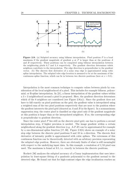
28 CHAPTER 2. TECHNICAL BACKGROUND (a) 300 250 200 150 100 50 0 Interpolated subpixel edge location Discrete 1st derivative Spline Interpolation Edge Profile 50 0 2 4 6 8 10 12 14 16 18 x Figure 2.9: (a) Subpixel accuracy using bilinear interpolation. Pixel position P is a local maximum if the gradient magnitude of gradient g at P is larger than at the positions A and B respectively. These positions can be computed using bilinear interpolation between the neighboring pixels 0, 7and3, 4 respectively. The gradient direction determines which neighbors contribute to the interpolation. The edge direction is perpendicular to the gradient vector. (b) The discrete first derivative of a noisy step edge is approximated using cubic spline interpolation. The subpixel tube edge location is assumed to be at the maximum of the continuous spline function, which can lie in between two discrete positions (here at x =9.5). Interpolation is the most common technique to compute values between pixels by consideration of the local neighborhood of a pixel. This includes for example bilinear, polynomial, or B-spline interpolation. In [21], a linear interpolation of the gradient values within a3× 3 neighborhood around a pixel is proposed. Here, the gradient direction determines whichofthe8neighborsareconsidered(seeFigure2.9(a)). Sincethegradientdoesnot have to fall exactly on pixel positions on the grid, the gradient value is interpolated using a weighted sum of the two pixel positions respectively that are next to the position where the gradient intersects the pixel grid (denoted as A and B in the figure). In a nonmaximum suppression step, the center pixel is classified as edge pixel only if the gradient magnitude at this position is larger than at the interpolated neighbors. If so, the corresponding edge is perpendicular to gradient direction. Since the center pixel P lies still on the discrete pixel grid, one has to perform a second interpolation step, if higher precision is needed. The image gradient within a certain neighborhood along the gradient direction (e.g. A-P -B) can be approximated for example by a one-dimensional spline function [17, 66]. Figure 2.9(b) shows an example of a noisy step edge between the discrete pixel positions 9 and 10 in x-direction. The discrete first derivative of intensity profile is approximated with cubic splines. The extremum of this continuous function can be theoretically detected with an arbitrary precision representing the subpixel edge position. However, there are obviously limits of what is still meaningful with respect to the underlying input data. In this example, a resolution of 1/10 pixel was used. The maximum is found at 9.5, i.e. exactly in between the discrete positions. Rockett [56] analyzes the subpixel accuracy of a Canny implementation that uses interpolation by least-square fitting of a quadratic polynomial to the gradient normal to the detected edge. He found out that for high-contrast edges the edge localization reaches an (b)
Page 1 and 2: Fachbereich Informatik Department o
Page 4: Acknowledgments First of all, I wou
Page 8 and 9: Contents Acknowledgments iii Abstra
Page 10 and 11: Contents ix 5.3.7. TubeLength .....
Page 12 and 13: List of Tables 1.1. Rangeoftubetype
Page 14 and 15: List of Figures 2.1. AccuracyandPre
Page 16 and 17: 1. Introduction Heat shrinkable tub
Page 18 and 19: 1.2. PROBLEM STATEMENT 3 hazards, r
Page 20 and 21: 1.4. RELATED WORK 5 Length [mm] Tol
Page 22 and 23: 1.5. THESIS OUTLINE 7 The vision pa
Page 24 and 25: 2. Technical Background 2.1. Visual
Page 26 and 27: 2.1. VISUAL MEASUREMENTS 11 (a) Fig
Page 28 and 29: 2.1. VISUAL MEASUREMENTS 13 Figure
Page 30 and 31: 2.1. VISUAL MEASUREMENTS 15 � xd
Page 32 and 33: 2.2. ILLUMINATION 17 tubes alternat
Page 34 and 35: 2.2. ILLUMINATION 19 effect of comp
Page 36 and 37: 2.3. EDGE DETECTION 21 i 2 i 1 0 (a
Page 38 and 39: 2.3. EDGE DETECTION 23 N × 1 kerne
Page 40 and 41: 2.3. EDGE DETECTION 25 These operat
Page 44 and 45: 2.4. TEMPLATE MATCHING 29 accuracy
Page 46 and 47: 3. Hardware Configuration This chap
Page 48 and 49: 3.2. CAMERA SETUP 33 3.2. Camera se
Page 50 and 51: 3.2. CAMERA SETUP 35 eachcolorchann
Page 52 and 53: 3.2. CAMERA SETUP 37 Figure 3.4: Co
Page 54 and 55: 3.2. CAMERA SETUP 39 adjusting scre
Page 56 and 57: 3.2. CAMERA SETUP 41 further distan
Page 58 and 59: 3.3. ILLUMINATION 43 f V 12mm 129mm
Page 60 and 61: 3.3. ILLUMINATION 45 (a) (b) (c) Fi
Page 62 and 63: 3.3. ILLUMINATION 47 (a) (b) Figure
Page 64 and 65: 3.4. BLOW OUT MECHANISM 49 A light
Page 66 and 67: 4. Length Measurement Approach Whil
Page 68 and 69: 4.2. MODEL KNOWLEDGE AND ASSUMPTION
Page 74 and 75: 4.3. CAMERA CALIBRATION 59 4.2.7. B
Page 76 and 77: 4.3. CAMERA CALIBRATION 61 Figure 4
Page 78 and 79: 4.3. CAMERA CALIBRATION 63 is compu
Page 80 and 81: 4.4. TUBE LOCALIZATION 65 (a) (b) F
Page 82 and 83: 4.4. TUBE LOCALIZATION 67 � 1 Psm
Page 84 and 85: 4.4. TUBE LOCALIZATION 69 Global Th
Page 86 and 87: 4.4. TUBE LOCALIZATION 71 but also
Page 88 and 89: 4.4. TUBE LOCALIZATION 73 Global Re
Page 90 and 91: 4.5. MEASURING POINT DETECTION 75 f
Page 92 and 93:
4.5. MEASURING POINT DETECTION 77 T
Page 94 and 95:
4.5. MEASURING POINT DETECTION 79 -
Page 96 and 97:
4.5. MEASURING POINT DETECTION 81 0
Page 98 and 99:
4.5. MEASURING POINT DETECTION 83 o
Page 100 and 101:
4.5. MEASURING POINT DETECTION 85 (
Page 102 and 103:
4.5. MEASURING POINT DETECTION 87 w
Page 104 and 105:
4.6. MEASURING 89 side of the tube,
Page 106 and 107:
4.6. MEASURING 91 fcor(x) =−(c1x
Page 108 and 109:
4.7. TEACH-IN 93 inthemeasuringplan
Page 110 and 111:
4.7. TEACH-IN 95 The pair of a pixe
Page 112 and 113:
5. Results and Evaluation 5.1. Expe
Page 114 and 115:
5.1. EXPERIMENTAL DESIGN 99 between
Page 116 and 117:
5.1. EXPERIMENTAL DESIGN 101 where
Page 118 and 119:
5.1. EXPERIMENTAL DESIGN 103 Ground
Page 120 and 121:
5.2. TEST SCENARIOS 105 enough, the
Page 122 and 123:
5.3. EXPERIMENTAL RESULTS 107 The t
Page 124 and 125:
5.3. EXPERIMENTAL RESULTS 109 Detec
Page 126 and 127:
5.3. EXPERIMENTAL RESULTS 111 Lengt
Page 128 and 129:
5.3. EXPERIMENTAL RESULTS 113 GTD [
Page 130 and 131:
5.3. EXPERIMENTAL RESULTS 115 gray
Page 132 and 133:
Page 134 and 135:
5.3. EXPERIMENTAL RESULTS 119 (a) (
Page 136 and 137:
5.3. EXPERIMENTAL RESULTS 121 (a) (
Page 138 and 139:
Page 140 and 141:
5.3. EXPERIMENTAL RESULTS 125 Total
Page 142 and 143:
5.3. EXPERIMENTAL RESULTS 127 Color
Page 144 and 145:
5.3. EXPERIMENTAL RESULTS 129 Task
Page 146 and 147:
5.4. DISCUSSION AND FUTURE WORK 131
Page 148 and 149:
6. Conclusion In this thesis a func
Page 150:
Appendix 135
Page 153 and 154:
138 APPENDIX A. PROFILE ANALYSIS IM
Page 155 and 156:
140 APPENDIX A. PROFILE ANALYSIS IM
Page 157 and 158:
142 APPENDIX B. HARDWARE COMPONENTS
Page 159 and 160:
144 APPENDIX B. HARDWARE COMPONENTS
Page 161 and 162:
146 Bibliography [18] C. Demant, B.
Page 163 and 164:
148 Bibliography [51] K.K. Pingle.
show all

Master Thesis - Fachbereich Informatik

You also want an ePaper? Increase the reach of your titles

Delete template?

Save as template?