- Page 2 and 3:
This text was adapted by The Saylor
- Page 4 and 5:
Chapter 1 Introductory Trade Issues
- Page 6 and 7:
However, rapid growth in the value
- Page 8 and 9:
As of 2009, 153 countries were memb
- Page 10 and 11:
International trade is a field in e
- Page 12 and 13:
imported, the U.S. government colle
- Page 14 and 15:
Kenya 12.7 Ghana 13.1 Generally spe
- Page 16 and 17:
Average tariffs can be measured as
- Page 18 and 19:
When the bubble bursts, the demand
- Page 20 and 21:
missed deadlines are commonplace in
- Page 22 and 23:
a well-known “bicycle theory” a
- Page 24 and 25:
But at the same time that many deve
- Page 26 and 27:
Recent opposition to trade liberali
- Page 28 and 29:
ought back to the United States and
- Page 30 and 31:
conference attended by the main all
- Page 32 and 33:
One of the key principles of the GA
- Page 34 and 35:
arriers. [1] The trade remedy laws
- Page 36 and 37:
ound tariff rate the country reache
- Page 38 and 39:
instead, they are put into place ov
- Page 40 and 41:
5. The WTO principle to treat an im
- Page 42 and 43:
subsidies. Recall that export subsi
- Page 44 and 45:
As a result of Uruguay Round negoti
- Page 46 and 47:
Agreement, or TRIPS. The TRIPS inte
- Page 48 and 49:
1.7 The World Trade Organization LE
- Page 50 and 51:
1. Consultations. The DSB first dem
- Page 52 and 53:
countries from choosing more destru
- Page 54 and 55:
P, P+ CAFTA-DR FTA PE MA OM R SG U.
- Page 56 and 57:
0806.10.20 $1.13/m 3 (Feb. 15-Mar.
- Page 58 and 59:
Tariffs vary according to time of e
- Page 60 and 61:
1.9 Appendix B: Bound versus Applie
- Page 62 and 63:
EXERCISE 1. Jeopardy Questions. As
- Page 64 and 65:
2.1 The Reasons for Trade LEARNING
- Page 66 and 67:
For example, the Ricardian model of
- Page 68 and 69:
2. Learn the major historical figur
- Page 70 and 71:
could end up with more of both good
- Page 72 and 73:
The primary issue in the analysis o
- Page 74 and 75:
Real wages (and incomes) of individ
- Page 76 and 77:
he begins planting seeds in the sec
- Page 78 and 79:
In this way, we might raise the wel
- Page 80 and 81:
2.3 Ricardian Model Assumptions LEA
- Page 82 and 83:
Utility Maximization and Demand In
- Page 84 and 85:
United States L C + L W = L France
- Page 86 and 87:
2. Suppose that the unit labor requ
- Page 88 and 89:
KEY TAKEAWAYS The equation aLC QC
- Page 90 and 91:
comparative advantage in newspaper
- Page 92 and 93:
−aLCaLW⎡⎣⎢hrslbhrsgal=gallb
- Page 94 and 95:
KEY TAKEAWAYS Labor productivity i
- Page 96 and 97:
2.6 A Ricardian Numerical Example L
- Page 98 and 99:
With full employment of labor, prod
- Page 100 and 101:
At this point, we can already see a
- Page 102 and 103:
The answer to some of these questio
- Page 104 and 105:
wC=PCaLC. If production occurs in t
- Page 106 and 107:
Thus a good way to think about how
- Page 108 and 109:
Similarly, by rearranging the above
- Page 110 and 111:
production. But where will they fin
- Page 112 and 113:
The focus on real wages allows us t
- Page 114 and 115:
Real Wages in Autarky To calculate
- Page 116 and 117:
exchange. Thus the real wage of che
- Page 118 and 119:
2.11 The Welfare Effects of Free Tr
- Page 120 and 121:
Free trade will raise aggregate wel
- Page 122 and 123:
Chapter 3 The Pure Exchange Model o
- Page 124 and 125:
A Simple Example of Trade Suppose t
- Page 126 and 127:
3.2 Determinants of the Terms of Tr
- Page 128 and 129:
Persuasion The art of persuasion ca
- Page 130 and 131:
KEY TAKEAWAY The terms of trade is
- Page 132 and 133:
two individuals make a voluntary ex
- Page 134 and 135:
3.4 Three Traders and Redistributio
- Page 136 and 137:
is not motivated by profit but inst
- Page 138 and 139:
The changes described above assume
- Page 140 and 141:
3.6 The Nondiscrimination Argument
- Page 142 and 143:
clothing worker. The same applies i
- Page 144 and 145:
the page, scroll down to the “Bou
- Page 146 and 147:
4.1 Factor Mobility Overview LEARNI
- Page 148 and 149: argument that free trade can only b
- Page 150 and 151: them, but only if the prices are ve
- Page 152 and 153: 4.3 Time and Factor Mobility LEARNI
- Page 154 and 155: EXERCISE 1. Jeopardy Questions. As
- Page 156 and 157: factor to be moved and become produ
- Page 158 and 159: KEY TAKEAWAY The immobile factor m
- Page 160 and 161: wine workers and cheese workers. Th
- Page 162 and 163: In autarky, the quantity demanded o
- Page 164 and 165: 4.7 Depicting a Free Trade Equilibr
- Page 166 and 167: 0 the variable does not change A th
- Page 168 and 169: Thus cheese workers are most likely
- Page 170 and 171: Real Wage of Wheat Workers in Terms
- Page 172 and 173: wages. However, these extra profits
- Page 174 and 175: EXERCISE 1. Jeopardy Questions. As
- Page 176 and 177: French production and consumption i
- Page 178 and 179: 5.1 Chapter Overview LEARNING OBJEC
- Page 180 and 181: less-developed countries have much
- Page 182 and 183: would rise, while the wage rate wou
- Page 184 and 185: Ricardian model, then factor prices
- Page 186 and 187: 4. This is by which industries diff
- Page 188 and 189: where KC and KS are the quantities
- Page 190 and 191: Let aLC[labor−hrsrack] represent
- Page 192 and 193: The capital-labor ratio in an indus
- Page 194 and 195: that would employ all the capital i
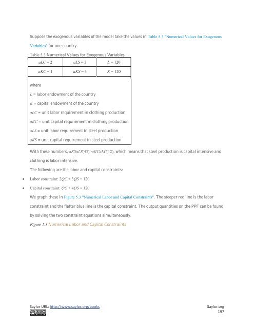
- Page 196 and 197: The Relationship between Endowments
- Page 200 and 201: Adding these two equations vertical
- Page 202 and 203: 3. Write the magnification effect f
- Page 204 and 205: tariffs or other government regulat
- Page 206 and 207: If the price of clothing had risen,
- Page 208 and 209: Table 5.6 Numerical Values for Exog
- Page 210 and 211: w∧>PC∧>PS∧>r∧. The effect i
- Page 212 and 213: 2. Suppose the price of cheese fall
- Page 214 and 215: this requires a fair amount of adva
- Page 216 and 217: workers per unit of capital in the
- Page 218 and 219: of quantities CS″/CC″. Since CS
- Page 220 and 221: In Figure 5.8 "Free Trade Equilibri
- Page 222 and 223: 5.11 National Welfare Effects of Fr
- Page 224 and 225: calculating changes in real income
- Page 226 and 227: who has deposits in a pension plan
- Page 228 and 229: export industry in order to benefit
- Page 230 and 231: Income is redistributed among indiv
- Page 232 and 233: Thus it is always possible to find
- Page 234 and 235: affects the capital-labor ratios in
- Page 236 and 237: 1. Describe the pattern of factor f
- Page 238 and 239: assumed to be freely and costlessly
- Page 240 and 241: expansion of output in the export s
- Page 242 and 243: [1] See R. W. Jones, “A Three-Fac
- Page 244 and 245: product line for a representative t
- Page 246 and 247: The total amount of revenue earned
- Page 248 and 249:
The horizontal length of Figure 5.1
- Page 250 and 251:
Our prime concern, however, is the
- Page 252 and 253:
An alternative version of the magni
- Page 254 and 255:
8. The magnification effect for pri
- Page 256 and 257:
can be used to transport tomatoes o
- Page 258 and 259:
esponds to the excess supply of wor
- Page 260 and 261:
The effect on workers is, in genera
- Page 262 and 263:
Factor Rewards over Time Now let’
- Page 264 and 265:
Figure 5.20 Dynamic Import-Capital
- Page 266 and 267:
In summary, the models suggest that
- Page 268 and 269:
[1] See J. P. Neary, “Short-Run C
- Page 270 and 271:
6.1 Chapter Overview LEARNING OBJEC
- Page 272 and 273:
6.2 Economies of Scale and Returns
- Page 274 and 275:
produced and if the costs of this e
- Page 276 and 277:
6.3 Gains from Trade with Economies
- Page 278 and 279:
United States aLC = 1 L = 100 Franc
- Page 280 and 281:
thirty racks of clothing, then each
- Page 282 and 283:
model best describes markets in whi
- Page 284 and 285:
2. Each firm produces a product tha
- Page 286 and 287:
2. The demand assumption in which e
- Page 288 and 289:
Keep in mind that this is the equil
- Page 290 and 291:
KEY TAKEAWAYS A market equilibrium
- Page 292 and 293:
1. If the product is such that an i
- Page 294 and 295:
varieties may increase aggregate we
- Page 296 and 297:
7.1 Basic Assumptions of the Partia
- Page 298 and 299:
2. The term used to describe a coun
- Page 300 and 301:
where XSUS(.) is the export supply
- Page 302 and 303:
This implies also that world supply
- Page 304 and 305:
1. The price that equalizes one cou
- Page 306 and 307:
The price that ultimately prevails
- Page 308 and 309:
Surplus", some firm would be willin
- Page 310 and 311:
Changes in Producer Surplus Suppose
- Page 312 and 313:
2. The term used to describe a meas
- Page 314 and 315:
the same price for their product re
- Page 316 and 317:
to purchase the Mexican wheat at $1
- Page 318 and 319:
The effect on the foreign price is
- Page 320 and 321:
The quantity of imports and exports
- Page 322 and 323:
the sum of the gains exceeds the su
- Page 324 and 325:
indicate the effect of each policy
- Page 326 and 327:
7.6 The Optimal Tariff LEARNING OBJ
- Page 328 and 329:
zero. Somewhere between a zero tari
- Page 330 and 331:
3. The tariff rate that corresponds
- Page 332 and 333:
KEY TAKEAWAYS An import tariff wil
- Page 334 and 335:
7.8 Import Tariffs: Small Country W
- Page 336 and 337:
3. The tariff causes a redistributi
- Page 338 and 339:
1. Where on the graph is the level
- Page 340 and 341:
We examine the effects of optimal t
- Page 342 and 343:
3. Given player one’s optimal pol
- Page 344 and 345:
The goal of a cooperative equilibri
- Page 346 and 347:
1. Use the information provided in
- Page 348 and 349:
7.10 Import Quotas: Large Country P
- Page 350 and 351:
An import quota will reduce the qua
- Page 352 and 353:
KEY TAKEAWAYS To administer a quot
- Page 354 and 355:
demand is equal to the quota level.
- Page 356 and 357:
market decreases producer surplus i
- Page 358 and 359:
Foreign National Welfare 2. Suppose
- Page 360 and 361:
This implies that, in the case of a
- Page 362 and 363:
Quota Rents National Welfare + C
- Page 364 and 365:
Import Quota (Administered by Givin
- Page 366 and 367:
to as tariffication. In this way, f
- Page 368 and 369:
Next, consider the effects in this
- Page 370 and 371:
In situations where market changes
- Page 372 and 373:
where S is the specific export subs
- Page 374 and 375:
7.17 Export Subsidies: Large Countr
- Page 376 and 377:
the subsidy payments are made, then
- Page 378 and 379:
An export subsidy of any size will
- Page 380 and 381:
2. Identify the effects of a counte
- Page 382 and 383:
Table 7.12 "Welfare Effects of the
- Page 384 and 385:
Consumer Surplus − (G + H + I + J
- Page 386 and 387:
KEY TAKEAWAYS An antisubsidy law,
- Page 388 and 389:
9. What is the change in government
- Page 390 and 391:
Notice that a unique set of prices
- Page 392 and 393:
in the import country and in the ca
- Page 394 and 395:
Figure 7.36 Welfare Effects of a VE
- Page 396 and 397:
the quota rents will benefit, but p
- Page 398 and 399:
A the variable change is ambiguous
- Page 400 and 401:
Mexico, and all wheat sold in Mexic
- Page 402 and 403:
7.23 Export Taxes: Large Country We
- Page 404 and 405:
Because there are both positive and
- Page 406 and 407:
− the variable decreases 0 the va
- Page 408 and 409:
8.1 Chapter Overview LEARNING OBJEC
- Page 410 and 411:
If a domestic consumption tax is im
- Page 412 and 413:
Equivalency between Domestic and Tr
- Page 414 and 415:
An import tariff applied on an impo
- Page 416 and 417:
KEY TAKEAWAYS Domestic production
- Page 418 and 419:
a Domestic Production Subsidy", whi
- Page 420 and 421:
Domestic policies can affect trade
- Page 422 and 423:
+ the variable increases − the va
- Page 424 and 425:
Domestic consumption taxes are ofte
- Page 426 and 427:
Figure 8.3 Inducing Exports with a
- Page 428 and 429:
8.7 Consumption Tax Effects in a Sm
- Page 430 and 431:
Since the cost to consumers exceeds
- Page 432 and 433:
When a specific consumption tax “
- Page 434 and 435:
time of the founding of the nation,
- Page 436 and 437:
Chapter 9 Trade Policies with Marke
- Page 438 and 439:
Market imperfections or market dist
- Page 440 and 441:
EXERCISE 1. Jeopardy Questions. As
- Page 442 and 443:
firm’s welfare) by restricting su
- Page 444 and 445:
are neatly kept and homes are well
- Page 446 and 447:
Policy-Imposed Distortions Another
- Page 448 and 449:
In this section, we will provide an
- Page 450 and 451:
Welfare-Improving Policies in a Sec
- Page 452 and 453:
Summary of the Theory of the Second
- Page 454 and 455:
9.4 Unemployment and Trade Policy L
- Page 456 and 457:
Suppose that international market c
- Page 458 and 459:
9.2 "Welfare Effects of an Import T
- Page 460 and 461:
Begin with the same surge of import
- Page 462 and 463:
eliminate the same unemployment imp
- Page 464 and 465:
A the variable change is ambiguous
- Page 466 and 467:
their own production efficiency imp
- Page 468 and 469:
Suppose that the infant industry ar
- Page 470 and 471:
This means that in the second perio
- Page 472 and 473:
The Economic Argument against Infan
- Page 474 and 475:
world efficiency standards, protect
- Page 476 and 477:
9.6 The Case of a Foreign Monopoly
- Page 478 and 479:
Assuming the monopolist maximizes p
- Page 480 and 481:
Import tariff effects on the import
- Page 482 and 483:
This shows that although a tariff c
- Page 484 and 485:
2. Recognize that a trade policy ca
- Page 486 and 487:
consider a large importing country
- Page 488 and 489:
the subsidy is set too high, the lo
- Page 490 and 491:
9.8 Public Goods and National Secur
- Page 492 and 493:
nonexcludable because once it is th
- Page 494 and 495:
efficiency loss. Nevertheless, the
- Page 496 and 497:
5. The term describing a ìgoodî l
- Page 498 and 499:
the environment. On the other hand,
- Page 500 and 501:
Pollution Effect National Welfare
- Page 502 and 503:
Govt. Revenue Pollution Effect + e
- Page 504 and 505:
A Source of Controversy For many en
- Page 506 and 507:
This statement points out that many
- Page 508 and 509:
noneconomists, providing permits th
- Page 510 and 511:
[4] World Trade Organization, “Tr
- Page 512 and 513:
product categories. This type of tr
- Page 514 and 515:
The key question of interest concer
- Page 516 and 517:
Figure 9.10 "Harmful Trade Diversio
- Page 518 and 519:
Free trade area effects on Country
- Page 520 and 521:
We assume that A has a specific tar
- Page 522 and 523:
The simple way to do that is to ima
- Page 524 and 525:
Chapter 10 Political Economy and In
- Page 526 and 527:
do indeed seek to maximize national
- Page 528 and 529:
a representative democracy, governm
- Page 530 and 531:
3. This type of lobbying does not i
- Page 532 and 533:
much larger than the number of firm
- Page 534 and 535:
We can now ask whether a household
- Page 536 and 537:
Large groups are much less effectiv
- Page 538 and 539:
Because the per-producer benefit of
- Page 540 and 541:
clearly he or she would vote for th
- Page 542 and 543:
10.7 The Lobbying Problem in a Demo
- Page 544 and 545:
Chapter 11 Evaluating the Controver
- Page 546 and 547:
the results from any one model. Ins
- Page 548 and 549:
increase in national welfare. This
- Page 550 and 551:
4. The enhancement of this is what
- Page 552 and 553:
of the real world. The real world c
- Page 554 and 555:
Another way to deflect the concern
- Page 556 and 557:
For example, an optimal tariff or o
- Page 558 and 559:
Stuart Mill in hisPrinciples of Pol
- Page 560 and 561:
11.5 The Economic Case against Sele
- Page 562 and 563:
to eliminate some of the inefficien
- Page 564 and 565:
effects, it would then need to meas
- Page 566 and 567:
to avoid the use of any such policy
- Page 568 and 569:
Selected protection requires detail
- Page 570 and 571:
11.6 Free Trade as the “Pragmatic