- Page 1 and 2:
Springer Tracts in Advanced Robotic
- Page 3 and 4:
Gianluca Antonelli Underwater Robot
- Page 5 and 6:
Editorial Advisory Board EUROPE Her
- Page 7 and 8:
Elalocomotiva sembrava fosse un mos
- Page 9 and 10:
Acknowledgements The contributions
- Page 11 and 12:
Preface to the Second Edition The p
- Page 13 and 14:
XVIII Preface to the First Edition
- Page 15 and 16:
XX Preface tothe First Edition mani
- Page 17 and 18:
XXII Notation η q =[η T 1 ε T η
- Page 19 and 20:
XXIV Notation ˜x error variable de
- Page 21 and 22:
XXVI Contents 3. Dynamic Control of
- Page 23 and 24:
XXVIIIContents A. Mathematical mode
- Page 25 and 26:
2 1. Introduction Maybe the first i
- Page 27 and 28:
4 1. Introduction (Massachusetts, U
- Page 29 and 30:
6 1. Introduction Fig. 1.4. Coordin
- Page 31 and 32:
8 1. Introduction Fig. 1.5. Pig, ma
- Page 33 and 34: 10 1. Introduction An example of cr
- Page 35 and 36: 12 1. Introduction Fig. 1.8. Romeo
- Page 37 and 38: 2. Modelling ofUnderwater Robots
- Page 39 and 40: 2.2 Rigid Body’s Kinematics 17 Th
- Page 41 and 42: J T k,oqJ k,oq = 1 4 I 3 , that all
- Page 43 and 44: 5. compute the quaternion Q by the
- Page 45 and 46: 2.3 Rigid Body’s Dynamics 23 Let
- Page 47 and 48: 2.4 Hydrodynamic Effects 25 τ 1 =
- Page 49 and 50: C A ( ν )=− C T A ( ν ) ∀ ν
- Page 51 and 52: 2.4 Hydrodynamic Effects 29 effects
- Page 53 and 54: 2.5 Gravity and Buoyancy 2.5 Gravit
- Page 55 and 56: 2.6 Thrusters’ Dynamics 33 Fig. 2
- Page 57 and 58: 2.7 Underwater Vehicles’ Dynamics
- Page 59 and 60: y z 2.8 Kinematics of Manipulators
- Page 61 and 62: 2.9 Dynamics ofUnderwater Vehicle-M
- Page 63 and 64: 2.9 Dynamics ofUnderwater Vehicle-M
- Page 65 and 66: 2.11 Identification 43 f e = K ( x
- Page 67 and 68: 3. Dynamic Control of 6-DOF AUVs 3.
- Page 69 and 70: 3.2 Earth-Fixed-Frame-Based, Model-
- Page 71 and 72: o x z o b z b x b 3.3 Earth-Fixed-F
- Page 73 and 74: 3.4 Vehicle-Fixed-Frame-Based, Mode
- Page 75 and 76: o o b y x y b x b 3.5 Model-Based C
- Page 77 and 78: 3.6 Mixed Earth/Vehicle-Fixed-Frame
- Page 79 and 80: 3.7 Jacobian-Transpose-Based Contro
- Page 81 and 82: 3.8 Comparison Among Controllers 59
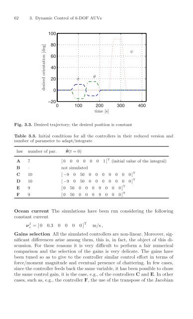
- Page 83: 3.9 Numerical Comparison Among the
- Page 87 and 88: force [N] moment [Nm] 20 10 0 −10
- Page 89 and 90: force [N] moment [Nm] 20 10 0 −10
- Page 91 and 92: force [N] moment [Nm] 20 10 0 −10
- Page 93 and 94: force [N] moment [Nm] 20 10 0 −10
- Page 95 and 96: force [N] moment [Nm] 20 10 0 −10
- Page 97 and 98: 3.9 Numerical Comparison Among the
- Page 99 and 100: 3.9 Numerical Comparison Among the
- Page 101 and 102: 80 4. Fault Detection/Tolerance Str
- Page 103 and 104: 82 4. Fault Detection/Tolerance Str
- Page 105 and 106: 84 4. Fault Detection/Tolerance Str
- Page 107 and 108: 86 4. Fault Detection/Tolerance Str
- Page 109 and 110: 88 4. Fault Detection/Tolerance Str
- Page 111 and 112: 90 4. Fault Detection/Tolerance Str
- Page 113 and 114: 5. Experiments of Dynamic Control o
- Page 115 and 116: 5.3 Experiments of Dynamic Control
- Page 117 and 118: [m] [m] 5 4 3 2 1 0 0 100 200 300 4
- Page 119 and 120: 5.3 Experiments of Dynamic Control
- Page 121 and 122: 5.4 Experiments of Fault Tolerance
- Page 123 and 124: [deg] 120 100 80 60 40 20 0 −20 5
- Page 125 and 126: 6. Kinematic Control of UVMSs “.
- Page 127 and 128: 6.2 Kinematic Control 107 UVMS. Thi
- Page 129 and 130: 6.2 Kinematic Control 109 singulari
- Page 131 and 132: 6.2 Kinematic Control 111 case of t
- Page 133 and 134: 6.5 Singularity-Robust Task Priorit
- Page 135 and 136:
6.5 Singularity-Robust Task Priorit
- Page 137 and 138:
6.5 Singularity-Robust Task Priorit
- Page 139 and 140:
6.5 Singularity-Robust Task Priorit
- Page 141 and 142:
6.6 Fuzzy Inverse Kinematics 121 It
- Page 143 and 144:
Simulations 6.6 Fuzzy Inverse Kinem
- Page 145 and 146:
6.6 Fuzzy Inverse Kinematics 125 Fi
- Page 147 and 148:
vehicle attitude [deg] 20 10 0 −1
- Page 149 and 150:
6.6 Fuzzy Inverse Kinematics 129 It
- Page 151 and 152:
[-] 1 0.8 0.6 0.4 0.2 0 close 0 20
- Page 153 and 154:
6.6 Fuzzy Inverse Kinematics 133 Fi
- Page 155 and 156:
joint positions 1-3 [deg] joint pos
- Page 157 and 158:
6.6 Fuzzy Inverse Kinematics 137 Fi
- Page 159 and 160:
e.e. position error [m] 0.02 0.01 0
- Page 161 and 162:
7. Dynamic Control of UVMSs 7.1 Int
- Page 163 and 164:
7.2 Feedforward Decoupling Control
- Page 165 and 166:
7.2 Feedforward Decoupling Control
- Page 167 and 168:
7.4 Nonlinear Control for UVMSs wit
- Page 169 and 170:
7.5 Non-regressor-Based Adaptive Co
- Page 171 and 172:
7.6 Sliding Mode Control 7.6 Slidin
- Page 173 and 174:
7.6 Sliding Mode Control 153 u = B
- Page 175 and 176:
7.6 Sliding Mode Control 155 Practi
- Page 177 and 178:
7.7 Adaptive Control 157 of gravity
- Page 179 and 180:
Let us consider the scalar function
- Page 181 and 182:
7.7 Adaptive Control 161 The vehicl
- Page 183 and 184:
[deg] 3 2.5 2 1.5 1 0.5 7.8 Output
- Page 185 and 186:
7.8 Output Feedback Control 165 It
- Page 187 and 188:
7.8 Output Feedback Control 167 whe
- Page 189 and 190:
7.8 Output Feedback Control 169 C T
- Page 191 and 192:
7.8 Output Feedback Control 171 wit
- Page 193 and 194:
[m] [deg] [deg] 0.1 0.05 0 −0.05
- Page 195 and 196:
[m] [-] [deg] x 10−3 10 8 6 4 2 0
- Page 197 and 198:
[Nm] [Nm] [Nm] 500 0 −500 50 0
- Page 199 and 200:
[m] [-] [deg] x 10−3 10 8 6 4 2 0
- Page 201 and 202:
[N] [N] [N] 20 0 −20 40 20 0 −2
- Page 203 and 204:
[Nm] [Nm] [Nm] 50 0 −50 350 300 2
- Page 205 and 206:
7.9 Virtual Decomposition Based Con
- Page 207 and 208:
7.9 Virtual Decomposition Based Con
- Page 209 and 210:
7.9 Virtual Decomposition Based Con
- Page 211 and 212:
7.9 Virtual Decomposition Based Con
- Page 213 and 214:
7.9 Virtual Decomposition Based Con
- Page 215 and 216:
joint torques [Nm] 200 0 −200 −
- Page 217 and 218:
e.e. orientation error [deg] 2 1 0
- Page 219 and 220:
vehicle position [m] 0.1 0.05 0 −
- Page 221 and 222:
8. Interaction Control of UVMSs 8.1
- Page 223 and 224:
8.3 Impedance Control 203 8.2 Dexte
- Page 225 and 226:
8.4 External Force Control 205 The
- Page 227 and 228:
8.4 External Force Control 207 be f
- Page 229 and 230:
8.4 External Force Control 209 that
- Page 231 and 232:
8.4 External Force Control 211 UVMS
- Page 233 and 234:
[N] [m] 350 300 250 200 150 100 50
- Page 235 and 236:
[deg] [deg] 10 5 0 −5 −10 50 40
- Page 237 and 238:
8.5 Explicit Force Control 217 wher
- Page 239 and 240:
8.5 Explicit Force Control 219 wher
- Page 241 and 242:
[m] [deg] 0.2 0.1 0 −0.1 8.5 Expl
- Page 243 and 244:
[m] [deg] 0.2 0.1 0 −0.1 −0.2 0
- Page 245 and 246:
226 9. Coordinated Control of Plato
- Page 247 and 248:
228 9. Coordinated Control of Plato
- Page 249 and 250:
230 9. Coordinated Control of Plato
- Page 251 and 252:
232 9. Coordinated Control of Plato
- Page 253 and 254:
234 9. Coordinated Control of Plato
- Page 255 and 256:
236 9. Coordinated Control of Plato
- Page 257 and 258:
238 10. Concluding Remarks control
- Page 259 and 260:
240 A. Mathematical models ⎡ 6 .
- Page 261 and 262:
242 A. Mathematical models using th
- Page 263 and 264:
244 A. Mathematical models L = 2 m
- Page 265 and 266:
References 1. Alekseev Y.K., Kosten
- Page 267 and 268:
References 249 28. Antonelli G.and
- Page 269 and 270:
References 251 62. Caccia M., Indiv
- Page 271 and 272:
References 253 96. Cui Y. and Sarka
- Page 273 and 274:
References 255 134. Garcia R., Puig
- Page 275 and 276:
References 257 168. Kato N. and Lan
- Page 277 and 278:
References 259 mera. In: IEEE Inter
- Page 279 and 280:
References 261 235. Podder T.K. and
- Page 281 and 282:
References 263 273. Solvang B., Den
- Page 283:
References 265 310. Yoerger D.R., S