- Page 2:
Fluid Mechanics, Thermodynamics of
- Page 6:
Preface to the Fifth Edition In the
- Page 10:
Preface to the Fourth Edition It is
- Page 14:
Preface to Third Edition Several mo
- Page 18:
List of Symbols A area A2 area of a
- Page 22:
z enthalpy loss coefficient, total
- Page 26:
Contents PREFACE TO THE FIFTH EDITI
- Page 30:
Velocity diagrams of the compressor
- Page 34:
10. Wind Turbines 323 Introduction
- Page 38:
2 Fluid Mechanics, Thermodynamics o
- Page 42:
4 Fluid Mechanics, Thermodynamics o
- Page 46:
6 Fluid Mechanics, Thermodynamics o
- Page 50:
8 Fluid Mechanics, Thermodynamics o
- Page 54:
10 Fluid Mechanics, Thermodynamics
- Page 58:
12 Fluid Mechanics, Thermodynamics
- Page 62:
14 Fluid Mechanics, Thermodynamics
- Page 66:
16 Fluid Mechanics, Thermodynamics
- Page 70:
18 Fluid Mechanics, Thermodynamics
- Page 74:
20 Fluid Mechanics, Thermodynamics
- Page 78:
22 Fluid Mechanics, Thermodynamics
- Page 82:
CHAPTER 2 Basic Thermodynamics, Flu
- Page 86:
26 Fluid Mechanics, Thermodynamics
- Page 90:
28 Fluid Mechanics, Thermodynamics
- Page 94:
30 Fluid Mechanics, Thermodynamics
- Page 98:
32 Fluid Mechanics, Thermodynamics
- Page 102:
34 Fluid Mechanics, Thermodynamics
- Page 106:
36 Fluid Mechanics, Thermodynamics
- Page 110:
38 Fluid Mechanics, Thermodynamics
- Page 114:
40 Fluid Mechanics, Thermodynamics
- Page 118:
42 Fluid Mechanics, Thermodynamics
- Page 122:
44 Fluid Mechanics, Thermodynamics
- Page 126:
46 Fluid Mechanics, Thermodynamics
- Page 130:
48 Fluid Mechanics, Thermodynamics
- Page 134:
50 Fluid Mechanics, Thermodynamics
- Page 138:
52 Fluid Mechanics, Thermodynamics
- Page 142:
54 Fluid Mechanics, Thermodynamics
- Page 146:
CHAPTER 3 Two-dimensional Cascades
- Page 150:
58 Fluid Mechanics, Thermodynamics
- Page 154:
60 Fluid Mechanics, Thermodynamics
- Page 158:
62 Fluid Mechanics, Thermodynamics
- Page 162:
64 Fluid Mechanics, Thermodynamics
- Page 166:
66 Fluid Mechanics, Thermodynamics
- Page 170:
68 Fluid Mechanics, Thermodynamics
- Page 174:
70 Fluid Mechanics, Thermodynamics
- Page 178:
72 Fluid Mechanics, Thermodynamics
- Page 182:
74 Fluid Mechanics, Thermodynamics
- Page 186:
76 Fluid Mechanics, Thermodynamics
- Page 190:
78 Fluid Mechanics, Thermodynamics
- Page 194:
80 Fluid Mechanics, Thermodynamics
- Page 198:
82 Fluid Mechanics, Thermodynamics
- Page 202:
84 Fluid Mechanics, Thermodynamics
- Page 206:
86 Fluid Mechanics, Thermodynamics
- Page 210:
88 Fluid Mechanics, Thermodynamics
- Page 214:
90 Fluid Mechanics, Thermodynamics
- Page 218:
92 Fluid Mechanics, Thermodynamics
- Page 222:
CHAPTER 4 Axial-flow Turbines: Two-
- Page 226:
96 Fluid Mechanics, Thermodynamics
- Page 230:
98 Fluid Mechanics, Thermodynamics
- Page 234:
100 Fluid Mechanics, Thermodynamics
- Page 238:
102 Fluid Mechanics, Thermodynamics
- Page 242:
104 Fluid Mechanics, Thermodynamics
- Page 246:
106 Fluid Mechanics, Thermodynamics
- Page 250:
108 Fluid Mechanics, Thermodynamics
- Page 254:
110 Fluid Mechanics, Thermodynamics
- Page 258:
112 Fluid Mechanics, Thermodynamics
- Page 262:
114 Fluid Mechanics, Thermodynamics
- Page 266:
116 Fluid Mechanics, Thermodynamics
- Page 270:
118 Fluid Mechanics, Thermodynamics
- Page 274:
120 Fluid Mechanics, Thermodynamics
- Page 278:
122 Fluid Mechanics, Thermodynamics
- Page 282:
124 Fluid Mechanics, Thermodynamics
- Page 286:
126 Fluid Mechanics, Thermodynamics
- Page 290:
128 Fluid Mechanics, Thermodynamics
- Page 294:
130 Fluid Mechanics, Thermodynamics
- Page 298:
132 Fluid Mechanics, Thermodynamics
- Page 302:
134 Fluid Mechanics, Thermodynamics
- Page 306:
136 Fluid Mechanics, Thermodynamics
- Page 310:
138 Fluid Mechanics, Thermodynamics
- Page 314:
140 Fluid Mechanics, Thermodynamics
- Page 318:
142 Fluid Mechanics, Thermodynamics
- Page 322:
144 Fluid Mechanics, Thermodynamics
- Page 326:
146 Fluid Mechanics, Thermodynamics
- Page 330:
148 Fluid Mechanics, Thermodynamics
- Page 334:
150 Fluid Mechanics, Thermodynamics
- Page 338:
152 Fluid Mechanics, Thermodynamics
- Page 342:
154 Fluid Mechanics, Thermodynamics
- Page 346:
156 Fluid Mechanics, Thermodynamics
- Page 350:
158 Fluid Mechanics, Thermodynamics
- Page 354: 160 Fluid Mechanics, Thermodynamics
- Page 358: 162 Fluid Mechanics, Thermodynamics
- Page 362: 164 Fluid Mechanics, Thermodynamics
- Page 366: 166 Fluid Mechanics, Thermodynamics
- Page 370: 168 Fluid Mechanics, Thermodynamics
- Page 374: 170 Fluid Mechanics, Thermodynamics
- Page 378: 172 Fluid Mechanics, Thermodynamics
- Page 382: 174 Fluid Mechanics, Thermodynamics
- Page 386: 176 Fluid Mechanics, Thermodynamics
- Page 390: 178 Fluid Mechanics, Thermodynamics
- Page 394: 180 Fluid Mechanics, Thermodynamics
- Page 398: 182 Fluid Mechanics, Thermodynamics
- Page 402: 184 Fluid Mechanics, Thermodynamics
- Page 408: where In the above example, 1 - a/W
- Page 412: therefore (6.24) For this free-vort
- Page 416: After differentiating the last term
- Page 420: (6.38) after combining with eqn. (6
- Page 424: Three-dimensional Flows in Axial Tu
- Page 428: velocity undergoes an abrupt change
- Page 432: adding these to the related radial
- Page 436: Three-dimensional Flows in Axial Tu
- Page 440: Three-dimensional Flows in Axial Tu
- Page 444: References Adamczyk, J. J. (2000).
- Page 448: and the axial velocity is constant
- Page 452: engine turbochargers, chemical plan
- Page 456:
Centrifugal Pumps, Fans and Compres
- Page 460:
or since Since I1 = I2 across the i
- Page 464:
For the inlet geometry shown in Fig
- Page 468:
The required diameter of the eye is
- Page 472:
(Mr1) = mW 2 /(p k p 01 a01 3 ) ·
- Page 476:
(iii) Use of prewhirl at entry to i
- Page 480:
(7.13a) where cq2 is the tangential
- Page 484:
Centrifugal Pumps, Fans and Compres
- Page 488:
(number of blades). He also found t
- Page 492:
Determining the velocities and head
- Page 496:
efficiencies seldom exceeded 80% gi
- Page 500:
Centrifugal Pumps, Fans and Compres
- Page 504:
efficiently converting this energy
- Page 508:
Therefore Hence, The diffuser syste
- Page 512:
Dq (deg) 240 160 80 Centrifugal Pum
- Page 516:
(7.41) If choking occurs in the rot
- Page 520:
Van den Braembussche, R. (1985). De
- Page 524:
Assuming that the hydraulic efficie
- Page 528:
Radial Flow Gas Turbines 247 FIG. 8
- Page 532:
Radial Flow Gas Turbines 249 FIG. 8
- Page 536:
Basic design of the rotor Radial Fl
- Page 540:
Radial Flow Gas Turbines 253 (8.9)
- Page 544:
Thus, the total-to-static efficienc
- Page 548:
Now, Loss coefficients in 90deg IFR
- Page 552:
P S P S c 2 Direction of rotation (
- Page 556:
and, combining this with eqns. (8.2
- Page 560:
(ii) Rewriting eqn. (8.26), (iii) U
- Page 564:
Thus, combining eqns. (8.39) and (8
- Page 568:
U 2/c o 0.8 0.7 0.6 88 Radial Flow
- Page 572:
(a) the static pressure at rotor ex
- Page 576:
(a) (2) (1) w 2 b2 ¢ w 2 ¢ b2, op
- Page 580:
Radial Flow Gas Turbines 273 This e
- Page 584:
Radial Flow Gas Turbines 275 FIG. 8
- Page 588:
Radial Flow Gas Turbines 277 FIG. 8
- Page 592:
Radial Flow Gas Turbines 279 occurs
- Page 596:
Radial Flow Gas Turbines 281 FIG. 8
- Page 600:
(a) f = 0.83 a 0 = q 0 U 0 = -7.18
- Page 604:
Measured performance Radial Flow Ga
- Page 608:
Radial Flow Gas Turbines 287 Whitfi
- Page 612:
Radial Flow Gas Turbines 289 Absolu
- Page 616:
Hydraulic Turbines 291 TABLE 9.1. D
- Page 620:
TABLE 9.3. Operating ranges of hydr
- Page 624:
Hydraulic Turbines 295 ridge splits
- Page 628:
Hydraulic Turbines 297 (9.3) (9.4)
- Page 632:
Hydraulic Turbines 299 FIG. 9.8. Me
- Page 636:
Hydraulic Turbines 301 (9.10) The e
- Page 640:
Neglecting bearing and windage loss
- Page 644:
Hydraulic Turbines 305 Figure 9.12
- Page 648:
Hydraulic Turbines 307 It is of int
- Page 652:
Hydraulic Turbines 309 constant. Th
- Page 656:
(a) (b) Hydraulic Turbines 311 FIG.
- Page 660:
TABLE 9.4. Calculated values of flo
- Page 664:
Hydraulic Turbines 315 gave measure
- Page 668:
Hydraulic Turbines 317 using Thoma
- Page 672:
Avoiding cavitation Hydraulic Turbi
- Page 676:
Hydraulic Turbines 321 nozzles. The
- Page 680:
CHAPTER 10 Wind Turbines Take care
- Page 684:
FIG. 10.2. Tower Windmill, Bidston,
- Page 688:
Brake discs Flexible coupling Build
- Page 692:
Small HAWTs Small wind turbines wit
- Page 696:
(iii) no flow rotation produced by
- Page 700:
It is convenient to define an axial
- Page 704:
Example 10.2. Determine the radii o
- Page 708:
where a - T = 0.3262. Sharpe (1990)
- Page 712:
each element must have an associate
- Page 716:
In the actuator disc analysis the v
- Page 720:
operate in post-stall conditions wh
- Page 724:
Solving the equations The foregoing
- Page 728:
Pitch angle, b (deg) 30 20 10 0 0.2
- Page 732:
TABLE 10.4. Data used for summing t
- Page 736:
F 1.0 0.8 0.6 0.4 0.2 0 0.4 dX = 4
- Page 740:
TABLE 10.5. Summary of results for
- Page 744:
Power coefficient, C P 0.6 0.4 0.2
- Page 748:
C X/(JC L) 0.14 0.12 0.10 0.08 0.06
- Page 752:
The flow angle j at optimum power c
- Page 756:
R 1 2 3 8 3 CP = P ( prR cx )= ( -a
- Page 760:
caused by this increased roughness
- Page 764:
Airfoil S820 S819 r/R 0.95 0.75 pro
- Page 768:
Airfoil S817 S816 r/R 0.95 0.75 NRE
- Page 772:
C C 0.4 0.2 -0 -0.2 -0.4 -0.6 twist
- Page 776:
According to Tangler (2002), some l
- Page 780:
understanding of the complex phenom
- Page 784:
References Wind Turbines 375 Abbott
- Page 788:
Bibliography Cumpsty, N. A. (1989).
- Page 792:
APPENDIX 2 Answers to Problems Chap
- Page 796:
Chapter 8 1. 586 m/s, 73.75 deg. 2.
- Page 800:
Index Terms Links Axial flow compre
- Page 804:
Index Terms Links Cascades, two-dim
- Page 808:
Index Terms Links Coefficient of, c
- Page 812:
Index Terms Links Diffusers (Cont.)
- Page 816:
Index Terms Links Francis turbine 2
- Page 820:
Index Terms Links Illustrative exam
- Page 824:
Index Terms Links Mollier diagram,
- Page 828:
Index Terms Links Pressure head 4 P
- Page 832:
Index Terms Links Rotor configurati
- Page 836:
Index Terms Links Thoma’s coeffic
- Page 840:
Index Terms Links U Units Imperial