multiple time scale dynamics with two fast variables and one slow ...

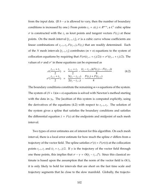
from the input data. (If b−a is allowed to vary, then the number of boundary
conditions is increased by one.) From points z j= z(t j)∈R m+n , a C 1 cubic spline
σ is constructed with the z j as knot points and tangent vectors F(z j) at these
points. On the mesh interval [t j−1, t j],σis a cubic curve whose coefficients are
linear combinations of z j−1, z j, F(z j−1), F(z j) that are readily determined. Each
of the N mesh intervals [t j−1, t j] contributes (m+n) equations to the system of
collocation equations by requiring that F(σ((t j−1+ t j)/2))=σ ′ ((t j−1+ t j)/2). The
values ofσandσ ′ in these equations can be expressed as
σ( t j−1+ t j
)
2
= z j−1+ z j
−
2
(t j− t j−1)(F(z j)− F(z j−1))
8
σ ′ ( t j−1+ t j
)
2
= 3(z j− z j−1)
2(t j− t j−1) − F(z j)+ F(z j−1)
4
(4.2)
The boundary conditions constitute the remaining m+n equations of the system.
The system of (N+ 1)(m+n) equations is solved with Newton’s method starting
with the data inγ0. The Jacobian of this system is computed explicitly, using
the derivatives of the equations (4.2) with respect to z j−1, z j. The solution of
the system gives a spline that satisfies the boundary conditions and satisfies
the differential equation ˙z=F(z) at the endpoints and midpoint of each mesh
interval.
Two types of error estimates are of interest for this algorithm. On each mesh
interval, there is a local error estimate for how much the splineσdiffers from a
trajectory of the vector field. The spline satisfiesσ ′ (t)=F(σ(t)) at the collocation
points t j−1, t j and (t j+ t j−1)/2. Ifγis the trajectory of the vector field through
one these points, this implies thatσ−γ=O(|t j− t j−1| 4 ). Since this classical es-
timate is based upon the assumption that the norm of the vector field is O(1),
it is only likely to hold for intervals that are short on the fast time scale and
trajectory segments that lie close to the slow manifold. Globally, the trajecto-
102