multiple time scale dynamics with two fast variables and one slow ...

More documents

Recommendations

Info

Note that we do not give a detailed description of dynamics associated to a singular Hopf bifurcation and refer the reader to the previous extensive litera- ture e.g. [4, 5, 13, 86, 52]. 6.3 Canard Explosion We describe the main results about canard explosion in fast-slow systems with one fast and one slow variable from [86]. Consider a planar fast-slow system of the form x ′ = f (x, y,λ,ǫ) y ′ = ǫg(x, y,λ,ǫ) (6.3) where f, g∈C k (R 4 , R) for k≥3,λ∈R is a parameter and 0 0 so that C0 is locally a parabola with a minimum at the origin. Using (6.4) and the implicit function theorem we have that C0 is the graph of a function y = φ(x) forφ : U → R where U is a sufficiently small neighborhood of x=0. Assume that C0 splits into an attracting and a repelling 149
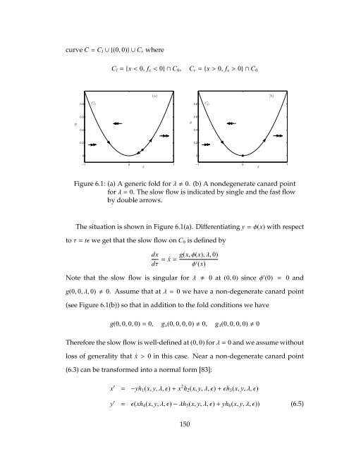
curve C= Cl∪{(0, 0)}∪ Cr where y 0.8 0.6 0.4 0.2 0 C0 C0 Cl={x0, fx> 0}∩ C0 −1 0 1 x x (a) (b) y y 0.8 0.6 0.4 0.2 0 C0 C0 −1 0 1 x Figure 6.1: (a) A generic fold forλ0. (b) A nondegenerate canard point forλ=0. The slow flow is indicated by single and the fast flow by double arrows. The situation is shown in Figure 6.1(a). Differentiating y=φ(x) with respect toτ=tǫ we get that the slow flow on C0 is defined by dx dτ = ˙x= g(x,φ(x),λ, 0) φ ′ (x) Note that the slow flow is singular forλ 0 at (0, 0) sinceφ ′ (0) = 0 and g(0, 0,λ, 0)0. Assume that atλ=0 we have a non-degenerate canard point (see Figure 6.1(b)) so that in addition to the fold conditions we have g(0, 0, 0, 0)=0, gx(0, 0, 0, 0)0, gλ(0, 0, 0, 0)0 Therefore the slow flow is well-defined at (0, 0) forλ=0 and we assume without loss of generality that ˙x>0 in this case. Near a non-degenerate canard point (6.3) can be transformed into a normal form [83]: x ′ = −yh1(x, y,λ,ǫ)+ x 2 h2(x, y,λ,ǫ)+ǫh3(x, y,λ,ǫ) y ′ = ǫ(xh4(x, y,λ,ǫ)−λh5(x, y,λ,ǫ)+yh6(x, y,λ,ǫ)) (6.5) 150 x
Page 1 and 2:
MULTIPLE TIME SCALE DYNAMICS WITH T
Page 3 and 4:
MULTIPLE TIME SCALE DYNAMICS WITH T
Page 5 and 6:
To my family. iv
Page 7 and 8:
ing mechanical systems.”, [E.T. P
Page 9 and 10:
TABLE OF CONTENTS Biographical Sket
Page 11 and 12:
LIST OF TABLES 5.1 Euclidean distan
Page 13 and 14:
3.1 Bifurcation diagram of (3.6). H
Page 15 and 16:
4.6 Boundary conditions are blue an
Page 17 and 18:
6.3 For all computations of the ful
Page 19 and 20:
where (x, y)∈R m × R n are varia
Page 21 and 22:
the general definition of normal hy
Page 23 and 24:
fast-slow system and yields: ˙x=(D
Page 25 and 26:
whereΛ,Γare matrix-valued functio
Page 27 and 28:
forǫ> 0. Therefore they have no im
Page 29 and 30:
The Hopf bifurcation is supercritic
Page 31 and 32:
where the algorithm can be used to
Page 33 and 34:
slow flow. In particular the manifo
Page 35 and 36:
f ast whereφ t is the flow of the
Page 37 and 38:
whereµ∈R p are parameters. Usual
Page 39 and 40:
We shall not prove this result but
Page 41 and 42:
d as given in equation (2.5). Let p
Page 43 and 44:
variables x1= u, x2= v and y=w we g
Page 45 and 46:
The geometry of the system for one
Page 47 and 48:
(0, 0, 0). 2.3 The Exchange Lemma I
Page 49 and 50:
withδ>0 sufficiently small. The sa
Page 51 and 52:
Theorem 2.3.2. Let ¯q ∈ M∩{|a|
Page 53 and 54:
exit point of a trajectory starting
Page 55 and 56:
Hence we have k=1=l and n=2 in view
Page 57 and 58:
The variational equations describin
Page 59 and 60:
(iii) Denote byη1i the i-th row of
Page 61 and 62:
Then let H(Z, X, t) := X ′ − BX
Page 63 and 64:
Proof. First, we work near q, then|
Page 65 and 66:
This result can be written more com
Page 67 and 68:
Proof. (of Theorem 2.4.2) The argum
Page 69 and 70:
ˆZ is still exponentially small. P
Page 71 and 72:
in the FitzHugh-Nagumo equation ǫ
Page 73 and 74:
center-unstable manifold W cu (0, 0
Page 75 and 76:
where the second “fast jump” oc
Page 77 and 78:
CHAPTER 3 PAPER I: “HOMOCLINIC OR
Page 79 and 80:
[39, 40, 41, 42]). It states that f
Page 81 and 82:
papers. Geometric singular perturba
Page 83 and 84:
s 2.2 2 1.8 1.6 1.4 1.2 1 0.8 0.6 0
Page 85 and 86:
One can view this as a projection o
Page 87 and 88:
for x1. We find that there are thre
Page 89 and 90:
We compute the functionsγl andγr
Page 91 and 92:
3.3.3 Two Slow Variables, One Fast
Page 93 and 94:
Also recall that the y-nullcline pa
Page 95 and 96:
is negative for all values h∈(0,
Page 97 and 98:
3.4 The Full System 3.4.1 Hopf Bifu
Page 99 and 100:
check whether this observation of a
Page 101 and 102:
indistinguishable numerically from
Page 103 and 104:
we should view this curve as an app
Page 105 and 106:
s 1.6 1.4 1.2 1 0.8 0.6 0.4 0.2 sin
Page 107 and 108:
waves” (see e.g. [63, 15, 69]). 3
Page 109 and 110:
the singular limits but it cannot b
Page 111 and 112:
Then (3.24) transforms to a three t
Page 113 and 114:
with x∈R m the vector of fast var
Page 115 and 116: ons that was used by David Terman i
Page 117 and 118: 0.15 0.1 0.05 0 −0.05 0.15 0.1 0.
Page 119 and 120: from the input data. (If b−a is a
Page 121 and 122: This explicit solution provides a b
Page 123 and 124: 4.4.2 Traveling Waves of the FitzHu
Page 125 and 126: computing the homoclinic orbit, eve
Page 127 and 128: y 0.15 0.1 0.05 0 −0.05 ε=0.001,
Page 129 and 130: eturns directly to q. Figure 4.5(b)
Page 131 and 132: are complicated [107]: we expect th
Page 133 and 134: t∈[0, 1]: z ′ = T F(z) H0(z(0))
Page 135 and 136: CHAPTER 5 PAPER III: “HOMOCLINIC
Page 137 and 138: s 1.6 1.4 1.2 1 0.8 0.6 0.4 0.2 0 H
Page 139 and 140: For a point p∈C0 we say that C0 i
Page 141 and 142: conjugate pair of eigenvalues for t
Page 143 and 144: Proof. (Sketch) The Lyapunov coeffi
Page 145 and 146: Table 5.1: Euclidean distance in (p
Page 147 and 148: gency of W s (q) with E u (Cl,ǫ).
Page 149 and 150: y x2 W s (q) C0 Cl,ǫ x1 W s (Cl,ǫ
Page 151 and 152: periodic orbit and q are restricted
Page 153 and 154: yΣ1=ψ(Σ1) andΣ2=ψ(Σ2); see Fi
Page 155 and 156: eigenvalues, Shilnikov [102] proved
Page 157 and 158: s 1.39 1.385 1.38 1.375 1.37 1.365
Page 159 and 160: Figure 5.9(a)-(b). It was obtained
Page 161 and 162: was carried out with the stiff solv
Page 163 and 164: 6.2 Introduction Our framework in t
Page 165: are called fold points. We can use
Page 169 and 170: explicitly. Note that currently no
Page 171 and 172: A slight modification of the formul
Page 173 and 174: 6.5 Relating l1 and K Krupa and Szm
Page 175 and 176: nates. The computer algebra system
Page 177 and 178: atλ=λH= 0 forǫ= 0.05 is l MC 1
Page 179 and 180: imum and maximum of the cubic. The
Page 181 and 182: 6.8 Additions It is important to no
Page 183 and 184: −7.85 −7.95 −8.05 λ x −7.9
Page 185 and 186: BIBLIOGRAPHY [1] V.I. Arnold. Encyc
Page 187 and 188: [26] M. Desroches, B. Krauskopf, an
Page 189 and 190: icated to Floris Takens. Eds.: Henk
Page 191 and 192: [74] T.J. Kaper and C.K.R.T. Jones.
Page 193: [98] H.G. Rotstein, M. Wechselberge
show all

multiple time scale dynamics with two fast variables and one slow ...

Create successful ePaper yourself

Delete template?

Save as template?