multiple time scale dynamics with two fast variables and one slow ...

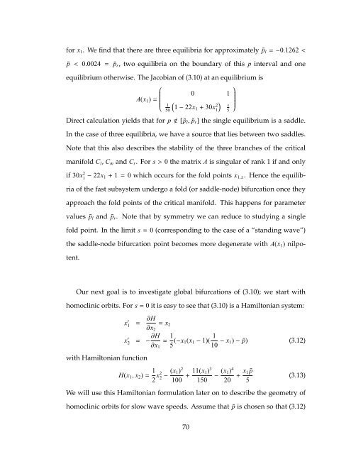
for x1. We find that there are three equilibria for approximately ¯pl=−0.1262<
¯p < 0.0024 = ¯pr, two equilibria on the boundary of this p interval and one
equilibrium otherwise. The Jacobian of (3.10) at an equilibrium is
⎛
0 1
A(x1)=
⎜⎝
1 1−22x1+ 30x 50
2
⎞
s ⎟⎠
1 5
Direct calculation yields that for p[ ¯pl, ¯pr] the single equilibrium is a saddle.
In the case of three equilibria, we have a source that lies between two saddles.
Note that this also describes the stability of the three branches of the critical
manifold Cl, Cm and Cr. For s>0 the matrix A is singular of rank 1 if and only
if 30x2 1− 22x1+ 1=0 which occurs for the fold points x1,±. Hence the equilibria
of the fast subsystem undergo a fold (or saddle-node) bifurcation once they
approach the fold points of the critical manifold. This happens for parameter
values ¯pl and ¯pr. Note that by symmetry we can reduce to studying a single
fold point. In the limit s=0 (corresponding to the case of a “standing wave”)
the saddle-node bifurcation point becomes more degenerate with A(x1) nilpo-
tent.
Our next goal is to investigate global bifurcations of (3.10); we start with
homoclinic orbits. For s=0 it is easy to see that (3.10) is a Hamiltonian system:
x ′
1
x ′
2
= ∂H
∂x2
with Hamiltonian function
= −∂H
∂x1
= x2
= 1
5 (−x1(x1− 1)( 1
10 − x1)− ¯p) (3.12)
H(x1, x2)= 1
2 x2
2
3 4
(x1) 11(x1) (x1)
2− + −
100 150 20 + x1 ¯p
5
(3.13)
We will use this Hamiltonian formulation later on to describe the geometry of
homoclinic orbits for slow wave speeds. Assume that ¯p is chosen so that (3.12)
70