- Page 1 and 2: MULTIPLE TIME SCALE DYNAMICS WITH T
- Page 3 and 4: MULTIPLE TIME SCALE DYNAMICS WITH T
- Page 5 and 6: To my family. iv
- Page 7 and 8: ing mechanical systems.”, [E.T. P
- Page 9 and 10: TABLE OF CONTENTS Biographical Sket
- Page 11 and 12: LIST OF TABLES 5.1 Euclidean distan
- Page 13 and 14: 3.1 Bifurcation diagram of (3.6). H
- Page 15 and 16: 4.6 Boundary conditions are blue an
- Page 17 and 18: 6.3 For all computations of the ful
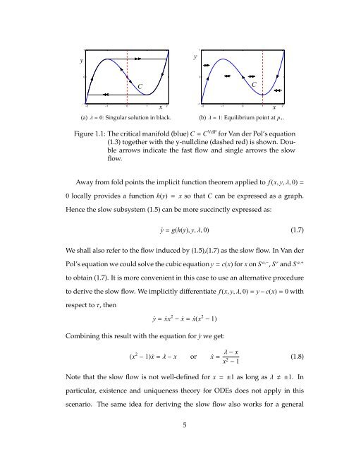
- Page 19 and 20: where (x, y)∈R m × R n are varia
- Page 21: the general definition of normal hy
- Page 25 and 26: whereΛ,Γare matrix-valued functio
- Page 27 and 28: forǫ> 0. Therefore they have no im
- Page 29 and 30: The Hopf bifurcation is supercritic
- Page 31 and 32: where the algorithm can be used to
- Page 33 and 34: slow flow. In particular the manifo
- Page 35 and 36: f ast whereφ t is the flow of the
- Page 37 and 38: whereµ∈R p are parameters. Usual
- Page 39 and 40: We shall not prove this result but
- Page 41 and 42: d as given in equation (2.5). Let p
- Page 43 and 44: variables x1= u, x2= v and y=w we g
- Page 45 and 46: The geometry of the system for one
- Page 47 and 48: (0, 0, 0). 2.3 The Exchange Lemma I
- Page 49 and 50: withδ>0 sufficiently small. The sa
- Page 51 and 52: Theorem 2.3.2. Let ¯q ∈ M∩{|a|
- Page 53 and 54: exit point of a trajectory starting
- Page 55 and 56: Hence we have k=1=l and n=2 in view
- Page 57 and 58: The variational equations describin
- Page 59 and 60: (iii) Denote byη1i the i-th row of
- Page 61 and 62: Then let H(Z, X, t) := X ′ − BX
- Page 63 and 64: Proof. First, we work near q, then|
- Page 65 and 66: This result can be written more com
- Page 67 and 68: Proof. (of Theorem 2.4.2) The argum
- Page 69 and 70: ˆZ is still exponentially small. P
- Page 71 and 72: in the FitzHugh-Nagumo equation ǫ
- Page 73 and 74:
center-unstable manifold W cu (0, 0
- Page 75 and 76:
where the second “fast jump” oc
- Page 77 and 78:
CHAPTER 3 PAPER I: “HOMOCLINIC OR
- Page 79 and 80:
[39, 40, 41, 42]). It states that f
- Page 81 and 82:
papers. Geometric singular perturba
- Page 83 and 84:
s 2.2 2 1.8 1.6 1.4 1.2 1 0.8 0.6 0
- Page 85 and 86:
One can view this as a projection o
- Page 87 and 88:
for x1. We find that there are thre
- Page 89 and 90:
We compute the functionsγl andγr
- Page 91 and 92:
3.3.3 Two Slow Variables, One Fast
- Page 93 and 94:
Also recall that the y-nullcline pa
- Page 95 and 96:
is negative for all values h∈(0,
- Page 97 and 98:
3.4 The Full System 3.4.1 Hopf Bifu
- Page 99 and 100:
check whether this observation of a
- Page 101 and 102:
indistinguishable numerically from
- Page 103 and 104:
we should view this curve as an app
- Page 105 and 106:
s 1.6 1.4 1.2 1 0.8 0.6 0.4 0.2 sin
- Page 107 and 108:
waves” (see e.g. [63, 15, 69]). 3
- Page 109 and 110:
the singular limits but it cannot b
- Page 111 and 112:
Then (3.24) transforms to a three t
- Page 113 and 114:
with x∈R m the vector of fast var
- Page 115 and 116:
ons that was used by David Terman i
- Page 117 and 118:
0.15 0.1 0.05 0 −0.05 0.15 0.1 0.
- Page 119 and 120:
from the input data. (If b−a is a
- Page 121 and 122:
This explicit solution provides a b
- Page 123 and 124:
4.4.2 Traveling Waves of the FitzHu
- Page 125 and 126:
computing the homoclinic orbit, eve
- Page 127 and 128:
y 0.15 0.1 0.05 0 −0.05 ε=0.001,
- Page 129 and 130:
eturns directly to q. Figure 4.5(b)
- Page 131 and 132:
are complicated [107]: we expect th
- Page 133 and 134:
t∈[0, 1]: z ′ = T F(z) H0(z(0))
- Page 135 and 136:
CHAPTER 5 PAPER III: “HOMOCLINIC
- Page 137 and 138:
s 1.6 1.4 1.2 1 0.8 0.6 0.4 0.2 0 H
- Page 139 and 140:
For a point p∈C0 we say that C0 i
- Page 141 and 142:
conjugate pair of eigenvalues for t
- Page 143 and 144:
Proof. (Sketch) The Lyapunov coeffi
- Page 145 and 146:
Table 5.1: Euclidean distance in (p
- Page 147 and 148:
gency of W s (q) with E u (Cl,ǫ).
- Page 149 and 150:
y x2 W s (q) C0 Cl,ǫ x1 W s (Cl,ǫ
- Page 151 and 152:
periodic orbit and q are restricted
- Page 153 and 154:
yΣ1=ψ(Σ1) andΣ2=ψ(Σ2); see Fi
- Page 155 and 156:
eigenvalues, Shilnikov [102] proved
- Page 157 and 158:
s 1.39 1.385 1.38 1.375 1.37 1.365
- Page 159 and 160:
Figure 5.9(a)-(b). It was obtained
- Page 161 and 162:
was carried out with the stiff solv
- Page 163 and 164:
6.2 Introduction Our framework in t
- Page 165 and 166:
are called fold points. We can use
- Page 167 and 168:
curve C= Cl∪{(0, 0)}∪ Cr where
- Page 169 and 170:
explicitly. Note that currently no
- Page 171 and 172:
A slight modification of the formul
- Page 173 and 174:
6.5 Relating l1 and K Krupa and Szm
- Page 175 and 176:
nates. The computer algebra system
- Page 177 and 178:
atλ=λH= 0 forǫ= 0.05 is l MC 1
- Page 179 and 180:
imum and maximum of the cubic. The
- Page 181 and 182:
6.8 Additions It is important to no
- Page 183 and 184:
−7.85 −7.95 −8.05 λ x −7.9
- Page 185 and 186:
BIBLIOGRAPHY [1] V.I. Arnold. Encyc
- Page 187 and 188:
[26] M. Desroches, B. Krauskopf, an
- Page 189 and 190:
icated to Floris Takens. Eds.: Henk
- Page 191 and 192:
[74] T.J. Kaper and C.K.R.T. Jones.
- Page 193:
[98] H.G. Rotstein, M. Wechselberge