multiple time scale dynamics with two fast variables and one slow ...

More documents

Recommendations

Info

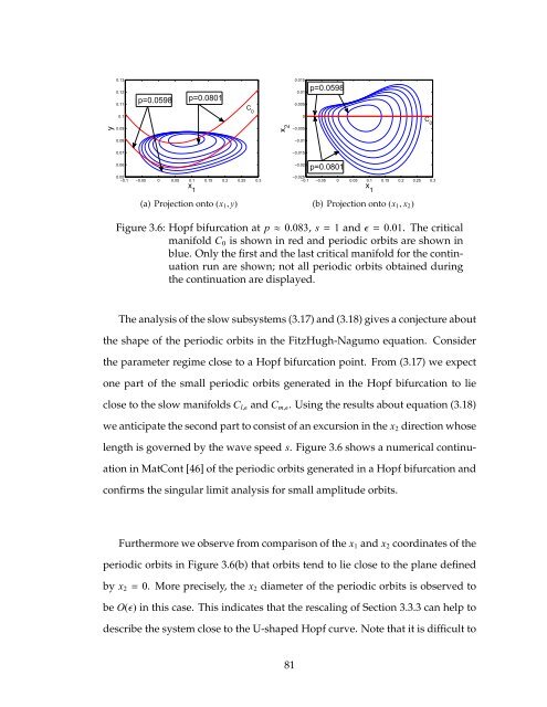
y 0.13 0.12 0.11 0.1 0.09 0.08 0.07 0.06 p=0.0598 p=0.0801 0.05 −0.1 −0.05 0 0.05 0.1 0.15 0.2 0.25 0.3 x 1 (a) Projection onto (x1, y) C 0 x 2 0.015 0.01 0.005 0 −0.005 −0.01 −0.015 −0.02 p=0.0598 p=0.0801 −0.025 −0.1 −0.05 0 0.05 0.1 0.15 0.2 0.25 0.3 x 1 (b) Projection onto (x1, x2) Figure 3.6: Hopf bifurcation at p≈0.083, s=1 andǫ= 0.01. The critical manifold C0 is shown in red and periodic orbits are shown in blue. Only the first and the last critical manifold for the continuation run are shown; not all periodic orbits obtained during the continuation are displayed. The analysis of the slow subsystems (3.17) and (3.18) gives a conjecture about the shape of the periodic orbits in the FitzHugh-Nagumo equation. Consider the parameter regime close to a Hopf bifurcation point. From (3.17) we expect one part of the small periodic orbits generated in the Hopf bifurcation to lie close to the slow manifolds Cl,ǫ and Cm,ǫ. Using the results about equation (3.18) we anticipate the second part to consist of an excursion in the x2 direction whose length is governed by the wave speed s. Figure 3.6 shows a numerical continuation in MatCont [46] of the periodic orbits generated in a Hopf bifurcation and confirms the singular limit analysis for small amplitude orbits. Furthermore we observe from comparison of the x1 and x2 coordinates of the periodic orbits in Figure 3.6(b) that orbits tend to lie close to the plane defined by x2= 0. More precisely, the x2 diameter of the periodic orbits is observed to be O(ǫ) in this case. This indicates that the rescaling of Section 3.3.3 can help to describe the system close to the U-shaped Hopf curve. Note that it is difficult to 81 C 0
check whether this observation of an O(ǫ)-diameter in the x2-coordinate persists for values ofǫ< 0.01 since numerical continuation of canard-type periodic orbits is difficult to use for smallerǫ. s 0.7 0.6 0.5 0.4 0.3 0.2 0.1 ε=0.01 ε=10 −7 0 0.1706 0.1707 0.1708 0.1709 0.171 0.1711 0.1712 (a) GH ǫ 1 p s 4 3.95 3.9 3.85 3.8 ε=10 −7 ε=0.01 3.75 0.051 0.052 0.053 0.054 0.055 0.056 0.057 0.058 0.059 (b) GH ǫ 2 Figure 3.7: Tracking of two generalized Hopf points (GH) in (p, s,ǫ)parameter space. Each point in the figure corresponds to a different value ofǫ. The point GHǫ 1 in 3.7(a) corresponds to the point shown as a square in Figure 3.1 and the point GHǫ 2 in 3.7(b) is further up on the left branch of the U-curve and is not displayed in Figure 3.1. In contrast to this, it is easily possible to compute the U-shaped Hopf curve using numerical continuation for very small values ofǫ. We have used this possibility to track two generalized Hopf bifurcation points in three parameters (p, s,ǫ). The U-shaped Hopf curve has been computed by numerical continuation for a mesh of parameter values forǫ between 10 −2 and 10 −7 using MatCont [46]. The two generalized Hopf points GHǫ 1,2 on the left half of the U-curve were detected as codimension two points during each continuation run. The results of this “three-parameter continuation” are shown in Figure 3.7. The two generalized Hopf points depend onǫ and we find that their singular 82 p
Page 1 and 2:
MULTIPLE TIME SCALE DYNAMICS WITH T
Page 3 and 4:
MULTIPLE TIME SCALE DYNAMICS WITH T
Page 5 and 6:
To my family. iv
Page 7 and 8:
ing mechanical systems.”, [E.T. P
Page 9 and 10:
TABLE OF CONTENTS Biographical Sket
Page 11 and 12:
LIST OF TABLES 5.1 Euclidean distan
Page 13 and 14:
3.1 Bifurcation diagram of (3.6). H
Page 15 and 16:
4.6 Boundary conditions are blue an
Page 17 and 18:
6.3 For all computations of the ful
Page 19 and 20:
where (x, y)∈R m × R n are varia
Page 21 and 22:
the general definition of normal hy
Page 23 and 24:
fast-slow system and yields: ˙x=(D
Page 25 and 26:
whereΛ,Γare matrix-valued functio
Page 27 and 28:
forǫ> 0. Therefore they have no im
Page 29 and 30:
The Hopf bifurcation is supercritic
Page 31 and 32:
where the algorithm can be used to
Page 33 and 34:
slow flow. In particular the manifo
Page 35 and 36:
f ast whereφ t is the flow of the
Page 37 and 38:
whereµ∈R p are parameters. Usual
Page 39 and 40:
We shall not prove this result but
Page 41 and 42:
d as given in equation (2.5). Let p
Page 43 and 44:
variables x1= u, x2= v and y=w we g
Page 45 and 46:
The geometry of the system for one
Page 47 and 48: (0, 0, 0). 2.3 The Exchange Lemma I
Page 49 and 50: withδ>0 sufficiently small. The sa
Page 51 and 52: Theorem 2.3.2. Let ¯q ∈ M∩{|a|
Page 53 and 54: exit point of a trajectory starting
Page 55 and 56: Hence we have k=1=l and n=2 in view
Page 57 and 58: The variational equations describin
Page 59 and 60: (iii) Denote byη1i the i-th row of
Page 61 and 62: Then let H(Z, X, t) := X ′ − BX
Page 63 and 64: Proof. First, we work near q, then|
Page 65 and 66: This result can be written more com
Page 67 and 68: Proof. (of Theorem 2.4.2) The argum
Page 69 and 70: ˆZ is still exponentially small. P
Page 71 and 72: in the FitzHugh-Nagumo equation ǫ
Page 73 and 74: center-unstable manifold W cu (0, 0
Page 75 and 76: where the second “fast jump” oc
Page 77 and 78: CHAPTER 3 PAPER I: “HOMOCLINIC OR
Page 79 and 80: [39, 40, 41, 42]). It states that f
Page 81 and 82: papers. Geometric singular perturba
Page 83 and 84: s 2.2 2 1.8 1.6 1.4 1.2 1 0.8 0.6 0
Page 85 and 86: One can view this as a projection o
Page 87 and 88: for x1. We find that there are thre
Page 89 and 90: We compute the functionsγl andγr
Page 91 and 92: 3.3.3 Two Slow Variables, One Fast
Page 93 and 94: Also recall that the y-nullcline pa
Page 95 and 96: is negative for all values h∈(0,
Page 97: 3.4 The Full System 3.4.1 Hopf Bifu
Page 101 and 102: indistinguishable numerically from
Page 103 and 104: we should view this curve as an app
Page 105 and 106: s 1.6 1.4 1.2 1 0.8 0.6 0.4 0.2 sin
Page 107 and 108: waves” (see e.g. [63, 15, 69]). 3
Page 109 and 110: the singular limits but it cannot b
Page 111 and 112: Then (3.24) transforms to a three t
Page 113 and 114: with x∈R m the vector of fast var
Page 115 and 116: ons that was used by David Terman i
Page 117 and 118: 0.15 0.1 0.05 0 −0.05 0.15 0.1 0.
Page 119 and 120: from the input data. (If b−a is a
Page 121 and 122: This explicit solution provides a b
Page 123 and 124: 4.4.2 Traveling Waves of the FitzHu
Page 125 and 126: computing the homoclinic orbit, eve
Page 127 and 128: y 0.15 0.1 0.05 0 −0.05 ε=0.001,
Page 129 and 130: eturns directly to q. Figure 4.5(b)
Page 131 and 132: are complicated [107]: we expect th
Page 133 and 134: t∈[0, 1]: z ′ = T F(z) H0(z(0))
Page 135 and 136: CHAPTER 5 PAPER III: “HOMOCLINIC
Page 137 and 138: s 1.6 1.4 1.2 1 0.8 0.6 0.4 0.2 0 H
Page 139 and 140: For a point p∈C0 we say that C0 i
Page 141 and 142: conjugate pair of eigenvalues for t
Page 143 and 144: Proof. (Sketch) The Lyapunov coeffi
Page 145 and 146: Table 5.1: Euclidean distance in (p
Page 147 and 148: gency of W s (q) with E u (Cl,ǫ).
Page 149 and 150:
y x2 W s (q) C0 Cl,ǫ x1 W s (Cl,ǫ
Page 151 and 152:
periodic orbit and q are restricted
Page 153 and 154:
yΣ1=ψ(Σ1) andΣ2=ψ(Σ2); see Fi
Page 155 and 156:
eigenvalues, Shilnikov [102] proved
Page 157 and 158:
s 1.39 1.385 1.38 1.375 1.37 1.365
Page 159 and 160:
Figure 5.9(a)-(b). It was obtained
Page 161 and 162:
was carried out with the stiff solv
Page 163 and 164:
6.2 Introduction Our framework in t
Page 165 and 166:
are called fold points. We can use
Page 167 and 168:
curve C= Cl∪{(0, 0)}∪ Cr where
Page 169 and 170:
explicitly. Note that currently no
Page 171 and 172:
A slight modification of the formul
Page 173 and 174:
6.5 Relating l1 and K Krupa and Szm
Page 175 and 176:
nates. The computer algebra system
Page 177 and 178:
atλ=λH= 0 forǫ= 0.05 is l MC 1
Page 179 and 180:
imum and maximum of the cubic. The
Page 181 and 182:
6.8 Additions It is important to no
Page 183 and 184:
−7.85 −7.95 −8.05 λ x −7.9
Page 185 and 186:
BIBLIOGRAPHY [1] V.I. Arnold. Encyc
Page 187 and 188:
[26] M. Desroches, B. Krauskopf, an
Page 189 and 190:
icated to Floris Takens. Eds.: Henk
Page 191 and 192:
[74] T.J. Kaper and C.K.R.T. Jones.
Page 193:
[98] H.G. Rotstein, M. Wechselberge
show all

multiple time scale dynamics with two fast variables and one slow ...

You also want an ePaper? Increase the reach of your titles

Delete template?

Save as template?