multiple time scale dynamics with two fast variables and one slow ...

More documents

Recommendations

Info

(a) In the case when the slow flow is one-dimensional (y∈R) it seems to be very helpful (possibly essential) to rescale the vector field: x ′ = f (x, y,ǫ) y ′ = ǫg(x, y,ǫ) The slow flow will be normalized to unit speedǫtg(x, y,ǫ)↦→ ˜t so that: dx d˜t dy d˜t = f (x, y,ǫ) ǫg(x, y,ǫ) = 1 Note that it remains a question for future work how to access the influence of the re-scaling on the numerical method including the case of higher- dimensional slow manifolds (y∈R n , n>1). (b) The standard boundary value solvers in MatLab bvp4c and bvp5c [101] do not seem to be able to solve the problem, although the same boundary conditions and initial guess as for our scheme presented above were used. Note that it is unclear whether this is a problem on the implemen- tation, user or algorithmic side. In fact, for moderate values ofǫ= O(10 −2 ) we would expect that almost any standard 2-point boundary value solver should be able to solve for a trajectory in the slow manifold manifold. Furthermore a different strategy for the linear test problem (4.3) was imple- mented in AUTO [34]. First we re-write the fast-slow system as z ′ = F(z) where z=(x, y)∈R N and F= ( f,ǫg). Let T denote the final time of a trajectory and re-scale t↦→ tT. Then we consider the following boundary value problem for 115
t∈[0, 1]: z ′ = T F(z) H0(z(0)) = h0 (4.10) H1(z(1)) = h1 with (h0, h1)∈R N . The boundary conditions can be chosen as described in Sec- tion 4.3. The problem (4.10) is in the standard form for computations with AUTO using 2-parameter continuation with NICP=2 as NICP=NBC+NINT-NDIM+2; see the AUTO manual for details [34]. Note that for (4.10) the final time T has be- come a parameter. As a second parameter we parametrize the endpoint boundary condition h1= h1(α) withα∈R. The main idea of the method is illustrated in Figure 4.6. 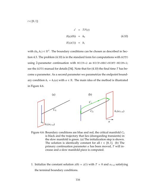C0 h0 h1(αT=0) (a) (b) Cǫ C0 α h1(αT>0) Figure 4.6: Boundary conditions are blue and red, the critical manifold C0 is black and the trajectory that lies (disregarding transients) in the slow manifold is green. (a) The initialization step is shown. The solution is identically constant for all t ∈ [0, 1]. (b) The primary continuation parameterαhas been moved, T will increase and a slow manifold piece is computed. 1. Initialize the constant solution z(0)=z(1) with T = 0 andαT=0 satisfying the terminal boundary conditions. 116
Page 1 and 2:
MULTIPLE TIME SCALE DYNAMICS WITH T
Page 3 and 4:
MULTIPLE TIME SCALE DYNAMICS WITH T
Page 5 and 6:
To my family. iv
Page 7 and 8:
ing mechanical systems.”, [E.T. P
Page 9 and 10:
TABLE OF CONTENTS Biographical Sket
Page 11 and 12:
LIST OF TABLES 5.1 Euclidean distan
Page 13 and 14:
3.1 Bifurcation diagram of (3.6). H
Page 15 and 16:
4.6 Boundary conditions are blue an
Page 17 and 18:
6.3 For all computations of the ful
Page 19 and 20:
where (x, y)∈R m × R n are varia
Page 21 and 22:
the general definition of normal hy
Page 23 and 24:
fast-slow system and yields: ˙x=(D
Page 25 and 26:
whereΛ,Γare matrix-valued functio
Page 27 and 28:
forǫ> 0. Therefore they have no im
Page 29 and 30:
The Hopf bifurcation is supercritic
Page 31 and 32:
where the algorithm can be used to
Page 33 and 34:
slow flow. In particular the manifo
Page 35 and 36:
f ast whereφ t is the flow of the
Page 37 and 38:
whereµ∈R p are parameters. Usual
Page 39 and 40:
We shall not prove this result but
Page 41 and 42:
d as given in equation (2.5). Let p
Page 43 and 44:
variables x1= u, x2= v and y=w we g
Page 45 and 46:
The geometry of the system for one
Page 47 and 48:
(0, 0, 0). 2.3 The Exchange Lemma I
Page 49 and 50:
withδ>0 sufficiently small. The sa
Page 51 and 52:
Theorem 2.3.2. Let ¯q ∈ M∩{|a|
Page 53 and 54:
exit point of a trajectory starting
Page 55 and 56:
Hence we have k=1=l and n=2 in view
Page 57 and 58:
The variational equations describin
Page 59 and 60:
(iii) Denote byη1i the i-th row of
Page 61 and 62:
Then let H(Z, X, t) := X ′ − BX
Page 63 and 64:
Proof. First, we work near q, then|
Page 65 and 66:
This result can be written more com
Page 67 and 68:
Proof. (of Theorem 2.4.2) The argum
Page 69 and 70:
ˆZ is still exponentially small. P
Page 71 and 72:
in the FitzHugh-Nagumo equation ǫ
Page 73 and 74:
center-unstable manifold W cu (0, 0
Page 75 and 76:
where the second “fast jump” oc
Page 77 and 78:
CHAPTER 3 PAPER I: “HOMOCLINIC OR
Page 79 and 80:
[39, 40, 41, 42]). It states that f
Page 81 and 82: papers. Geometric singular perturba
Page 83 and 84: s 2.2 2 1.8 1.6 1.4 1.2 1 0.8 0.6 0
Page 85 and 86: One can view this as a projection o
Page 87 and 88: for x1. We find that there are thre
Page 89 and 90: We compute the functionsγl andγr
Page 91 and 92: 3.3.3 Two Slow Variables, One Fast
Page 93 and 94: Also recall that the y-nullcline pa
Page 95 and 96: is negative for all values h∈(0,
Page 97 and 98: 3.4 The Full System 3.4.1 Hopf Bifu
Page 99 and 100: check whether this observation of a
Page 101 and 102: indistinguishable numerically from
Page 103 and 104: we should view this curve as an app
Page 105 and 106: s 1.6 1.4 1.2 1 0.8 0.6 0.4 0.2 sin
Page 107 and 108: waves” (see e.g. [63, 15, 69]). 3
Page 109 and 110: the singular limits but it cannot b
Page 111 and 112: Then (3.24) transforms to a three t
Page 113 and 114: with x∈R m the vector of fast var
Page 115 and 116: ons that was used by David Terman i
Page 117 and 118: 0.15 0.1 0.05 0 −0.05 0.15 0.1 0.
Page 119 and 120: from the input data. (If b−a is a
Page 121 and 122: This explicit solution provides a b
Page 123 and 124: 4.4.2 Traveling Waves of the FitzHu
Page 125 and 126: computing the homoclinic orbit, eve
Page 127 and 128: y 0.15 0.1 0.05 0 −0.05 ε=0.001,
Page 129 and 130: eturns directly to q. Figure 4.5(b)
Page 131: are complicated [107]: we expect th
Page 135 and 136: CHAPTER 5 PAPER III: “HOMOCLINIC
Page 137 and 138: s 1.6 1.4 1.2 1 0.8 0.6 0.4 0.2 0 H
Page 139 and 140: For a point p∈C0 we say that C0 i
Page 141 and 142: conjugate pair of eigenvalues for t
Page 143 and 144: Proof. (Sketch) The Lyapunov coeffi
Page 145 and 146: Table 5.1: Euclidean distance in (p
Page 147 and 148: gency of W s (q) with E u (Cl,ǫ).
Page 149 and 150: y x2 W s (q) C0 Cl,ǫ x1 W s (Cl,ǫ
Page 151 and 152: periodic orbit and q are restricted
Page 153 and 154: yΣ1=ψ(Σ1) andΣ2=ψ(Σ2); see Fi
Page 155 and 156: eigenvalues, Shilnikov [102] proved
Page 157 and 158: s 1.39 1.385 1.38 1.375 1.37 1.365
Page 159 and 160: Figure 5.9(a)-(b). It was obtained
Page 161 and 162: was carried out with the stiff solv
Page 163 and 164: 6.2 Introduction Our framework in t
Page 165 and 166: are called fold points. We can use
Page 167 and 168: curve C= Cl∪{(0, 0)}∪ Cr where
Page 169 and 170: explicitly. Note that currently no
Page 171 and 172: A slight modification of the formul
Page 173 and 174: 6.5 Relating l1 and K Krupa and Szm
Page 175 and 176: nates. The computer algebra system
Page 177 and 178: atλ=λH= 0 forǫ= 0.05 is l MC 1
Page 179 and 180: imum and maximum of the cubic. The
Page 181 and 182: 6.8 Additions It is important to no
Page 183 and 184:
−7.85 −7.95 −8.05 λ x −7.9
Page 185 and 186:
BIBLIOGRAPHY [1] V.I. Arnold. Encyc
Page 187 and 188:
[26] M. Desroches, B. Krauskopf, an
Page 189 and 190:
icated to Floris Takens. Eds.: Henk
Page 191 and 192:
[74] T.J. Kaper and C.K.R.T. Jones.
Page 193:
[98] H.G. Rotstein, M. Wechselberge
show all

multiple time scale dynamics with two fast variables and one slow ...

Create successful ePaper yourself

Delete template?

Save as template?