multiple time scale dynamics with two fast variables and one slow ...

manifold D0 of (3.18) is:
D0={(x1, ¯x2)∈R 2 : s ¯x2c ′ (x1)= x1− c(x1)}
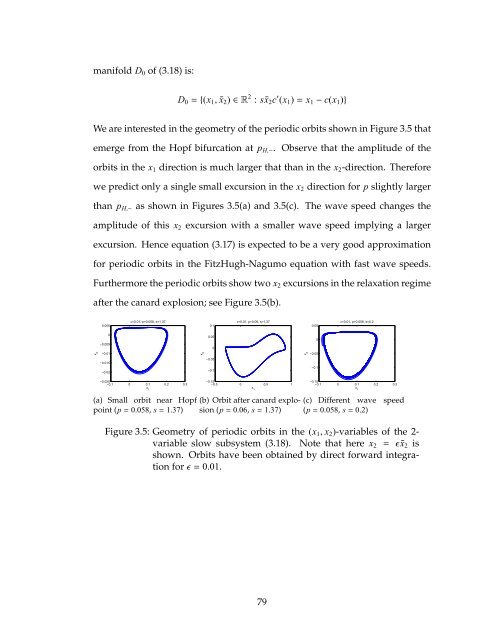
We are interested in the geometry of the periodic orbits shown in Figure 3.5 that
emerge from the Hopf bifurcation at pH,−. Observe that the amplitude of the
orbits in the x1 direction is much larger that than in the x2-direction. Therefore
we predict only a single small excursion in the x2 direction for p slightly larger
than pH,− as shown in Figures 3.5(a) and 3.5(c). The wave speed changes the
amplitude of this x2 excursion with a smaller wave speed implying a larger
excursion. Hence equation (3.17) is expected to be a very good approximation
for periodic orbits in the FitzHugh-Nagumo equation with fast wave speeds.
Furthermore the periodic orbits show two x2 excursions in the relaxation regime
after the canard explosion; see Figure 3.5(b).
x 2
0.005
0
−0.005
−0.01
−0.015
−0.02
ε=0.01, p=0.058, s=1.37
−0.025
−0.1 0 0.1
x
1
0.2 0.3
(a) Small orbit near Hopf
point (p=0.058, s=1.37)
x 2
0.1
0.05
0
−0.05
−0.1
ε=0.01, p=0.06, s=1.37
−0.15
−0.5 0 0.5 1
x
1
(b) Orbit after canard explosion
(p=0.06, s=1.37)
x 2
0.05
0
−0.05
−0.1
ε=0.01, p=0.058, s=0.2
−0.15
−0.1 0 0.1
x
1
0.2 0.3
(c) Different wave speed
(p=0.058, s=0.2)
Figure 3.5: Geometry of periodic orbits in the (x1, x2)-variables of the 2variable
slow subsystem (3.18). Note that here x2 = ǫ ¯x2 is
shown. Orbits have been obtained by direct forward integration
forǫ= 0.01.
79