multiple time scale dynamics with two fast variables and one slow ...

ory implies that a perturbed singular “slow” homoclinic orbit persists forǫ> 0
[103]. Again it is possible to compute parameter values (p1, s1) at which ho-
moclinic orbits forǫ> 0 exist [56]. To compute the orbits themselves a similar
approach as described above can be used. We have to track when W u (q) enters
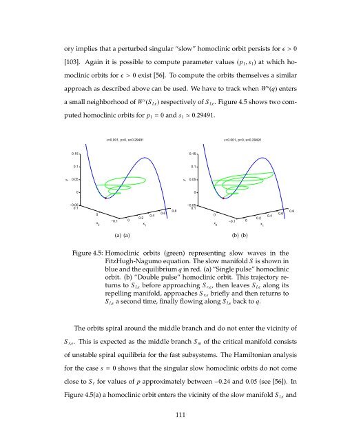
a small neighborhood of W s (S l,ǫ) respectively of S l,ǫ. Figure 4.5 shows two com-
puted homoclinic orbits for p1= 0 and s1≈ 0.29491.
y
0.15
0.1
0.05
0
−0.05
0.1
0
x 2
ε=0.001, p=0, s=0.29491
−0.1
0
(a) (a)
0.2
x 1
0.4
0.6
0.8
y
0.15
0.1
0.05
0
−0.05
0.1
0
x 2
ε=0.001, p=0, s=0.29491
−0.1
0
(b) (b)
Figure 4.5: Homoclinic orbits (green) representing slow waves in the
FitzHugh-Nagumo equation. The slow manifold S is shown in
blue and the equilibrium q in red. (a) “Single pulse” homoclinic
orbit. (b) “Double pulse” homoclinic orbit. This trajectory returns
to S l,ǫ before approaching S r,ǫ, then leaves S l,ǫ along its
repelling manifold, approaches S r,ǫ briefly and then returns to
S l,ǫ a second time, finally flowing along S l,ǫ back to q.
The orbits spiral around the middle branch and do not enter the vicinity of
S r,ǫ. This is expected as the middle branch S m of the critical manifold consists
of unstable spiral equilibria for the fast subsystems. The Hamiltonian analysis
for the case s=0 shows that the singular slow homoclinic orbits do not come
close to S r for values of p approximately between−0.24 and 0.05 (see [56]). In
Figure 4.5(a) a homoclinic orbit enters the vicinity of the slow manifold S l,ǫ and
111
0.2
x 1
0.4
0.6
0.8