- Page 1:
Pictures Paths Particles Processes
- Page 4 and 5:
4 CONTENTS 1.5.1 The effective acti
- Page 6 and 7:
6 CONTENTS 5.3.7 Massless Dirac par
- Page 8 and 9:
8 CONTENTS 9.3.3 W, Z and γ four-p
- Page 10 and 11:
10 November 7, 2013
- Page 12 and 13:
12 November 7, 2013 the like. The m
- Page 14 and 15:
14 November 7, 2013 cay widths. The
- Page 16 and 17:
16 November 7, 2013 scenario of a s
- Page 18 and 19:
18 November 7, 2013 which yields th
- Page 20 and 21:
20 November 7, 2013
- Page 22 and 23:
22 November 7, 2013 The function S(
- Page 24 and 25:
24 November 7, 2013 For a single-fi
- Page 26 and 27:
26 November 7, 2013 Computing the p
- Page 28 and 29:
28 November 7, 2013 Using the serie
- Page 30 and 31:
30 November 7, 2013 multiplied. The
- Page 32 and 33:
32 November 7, 2013 carries a symme
- Page 34 and 35:
34 November 7, 2013 therefore also
- Page 36 and 37:
000000 111111 000000 111111 000000
- Page 38 and 39:
38 November 7, 2013 1.4 Planck’s
- Page 40 and 41:
0000000 1111111 0000000 1111111 000
- Page 42 and 43:
42 November 7, 2013 1.4.3 The class
- Page 44 and 45:
44 November 7, 2013 Such subdominan
- Page 46 and 47:
000000 111111 000000 111111 000000
- Page 48 and 49:
48 November 7, 2013 diagrams. With
- Page 50 and 51:
50 November 7, 2013 with the follow
- Page 52 and 53:
52 November 7, 2013 1.6 Renormaliza
- Page 54 and 55:
54 November 7, 2013 C naive 2 C nai
- Page 56 and 57:
00000 11111 00000 11111 00000 11111
- Page 58 and 59:
58 November 7, 2013 We may formulat
- Page 60 and 61:
60 November 7, 2013 Using Eq.(1.136
- Page 62 and 63:
62 November 7, 2013 action has been
- Page 64 and 65:
64 November 7, 2013 zero-dimensiona
- Page 66 and 67:
66 November 7, 2013 The easiest way
- Page 68 and 69:
68 November 7, 2013 are deemed to b
- Page 70 and 71:
70 November 7, 2013 To check that t
- Page 72 and 73:
72 November 7, 2013 Upon ‘discret
- Page 74 and 75:
74 November 7, 2013 − λ 4 6 ( φ
- Page 76 and 77:
76 November 7, 2013 Here we plot a
- Page 78 and 79:
78 November 7, 2013 The continuum f
- Page 80 and 81:
80 November 7, 2013 For large m|⃗
- Page 82 and 83:
82 November 7, 2013 there is a law
- Page 84 and 85:
84 November 7, 2013 k ↔ ¯h | ⃗
- Page 86 and 87:
86 November 7, 2013 the integral is
- Page 88 and 89:
88 November 7, 2013 by (x − y) 2
- Page 90 and 91:
90 November 7, 2013 3.2.4 The iɛ p
- Page 92 and 93:
92 November 7, 2013 Im k 4 Re k 4 I
- Page 94 and 95:
94 November 7, 2013 The response of
- Page 96 and 97:
96 November 7, 2013 = 1 (2π) 3 ∫
- Page 98 and 99:
98 November 7, 2013 we find that th
- Page 100 and 101:
100 November 7, 2013 x x B B E > 0
- Page 102 and 103:
102 November 7, 2013 in which avail
- Page 104 and 105:
104 November 7, 2013 the time-evolu
- Page 106 and 107:
106 November 7, 2013 Now, the secon
- Page 108 and 109:
108 November 7, 2013 Note that the
- Page 110 and 111:
110 November 7, 2013 the story the
- Page 112 and 113:
112 November 7, 2013 The n-particle
- Page 114 and 115:
114 November 7, 2013 interactions.
- Page 116 and 117:
116 November 7, 2013 0000000 111111
- Page 118 and 119:
000000000 111111111 000000000 11111
- Page 120 and 121:
120 November 7, 2013 4.5.2 Two-body
- Page 122 and 123:
122 November 7, 2013 which, to lowe
- Page 124 and 125:
124 November 7, 2013
- Page 126 and 127:
126 November 7, 2013 Therefore, T (
- Page 128 and 129:
128 November 7, 2013 where Q is som
- Page 130 and 131:
130 November 7, 2013 (P ) coefficie
- Page 132 and 133:
132 November 7, 2013 Obviously, the
- Page 134 and 135:
134 November 7, 2013 Now, we also k
- Page 136 and 137:
136 November 7, 2013 p 2 = m 2 we c
- Page 138 and 139:
138 November 7, 2013 5.3.3 The Dira
- Page 140 and 141:
140 November 7, 2013 now forced by
- Page 142 and 143:
142 November 7, 2013 under Lorentz
- Page 144 and 145:
144 November 7, 2013 = 1 ( 1 + 1 (
- Page 146 and 147:
146 November 7, 2013 Dirac propagat
- Page 148 and 149:
148 November 7, 2013 The first diag
- Page 150 and 151:
150 November 7, 2013 5.5 The Dirac
- Page 152 and 153:
152 November 7, 2013 gives us preci
- Page 154 and 155:
154 November 7, 2013 this gives the
- Page 156 and 157:
156 November 7, 2013 and is picture
- Page 158 and 159:
158 November 7, 2013 5.7.3 The muon
- Page 160 and 161:
160 November 7, 2013 µ p ν ↔ i
- Page 162 and 163:
162 November 7, 2013 (T z ) µ ν =
- Page 164 and 165:
164 November 7, 2013 The SDe for a
- Page 166 and 167:
166 November 7, 2013 operator is th
- Page 168 and 169:
168 November 7, 2013 However, a pro
- Page 170 and 171:
170 November 7, 2013 transverse one
- Page 172 and 173:
172 November 7, 2013 in contrast to
- Page 174 and 175:
174 November 7, 2013
- Page 176 and 177:
176 November 7, 2013 µ ↔ iQ¯h
- Page 178 and 179:
178 November 7, 2013 the correspond
- Page 180 and 181:
180 November 7, 2013 The handlebar
- Page 182 and 183:
182 November 7, 2013 The Dirac equa
- Page 184 and 185:
184 November 7, 2013 7.3 Some QED p
- Page 186 and 187:
186 November 7, 2013 The cross sect
- Page 188 and 189:
188 November 7, 2013 We therefore h
- Page 190 and 191:
190 November 7, 2013 so that up to
- Page 192 and 193:
192 November 7, 2013 The radiative
- Page 194 and 195:
194 November 7, 2013 Hard Bremsstra
- Page 196 and 197:
196 November 7, 2013 Double-pole te
- Page 198 and 199:
198 November 7, 2013 with constants
- Page 200 and 201:
200 November 7, 2013 with the trivi
- Page 202 and 203:
202 November 7, 2013 7.4.4 The char
- Page 204 and 205:
204 November 7, 2013 positronium ma
- Page 206 and 207:
206 November 7, 2013 We now postula
- Page 208 and 209:
208 November 7, 2013 For the QED di
- Page 210 and 211:
210 November 7, 2013 8.3 The three-
- Page 212 and 213:
212 November 7, 2013 be renormaliza
- Page 214 and 215:
214 November 7, 2013 Also, in the a
- Page 216 and 217:
216 November 7, 2013 8.4 Four-gluon
- Page 218 and 219:
218 November 7, 2013 so that A 34 t
- Page 220 and 221:
220 November 7, 2013 We can therefo
- Page 222 and 223:
222 November 7, 2013 by p Q q k 1 k
- Page 224 and 225:
224 November 7, 2013 However, from
- Page 226 and 227:
226 November 7, 2013 If we were all
- Page 228 and 229:
228 November 7, 2013 with Z α as i
- Page 230 and 231:
230 November 7, 2013 ¯hQ U Q W M 2
- Page 232 and 233:
232 November 7, 2013 the process UU
- Page 234 and 235:
234 November 7, 2013 we have pretty
- Page 236 and 237:
236 November 7, 2013 where X µνα
- Page 238 and 239:
238 November 7, 2013 9.4 The Higgs
- Page 240 and 241:
240 November 7, 2013 in any dynamic
- Page 242 and 243:
242 November 7, 2013 with the contr
- Page 244 and 245:
244 November 7, 2013 remain unaffec
- Page 246 and 247:
246 November 7, 2013 Note that the
- Page 248 and 249:
248 November 7, 2013 following type
- Page 250 and 251:
250 November 7, 2013 + B 1 (1, 2, 5
- Page 252 and 253:
252 November 7, 2013
- Page 254 and 255: 254 November 7, 2013 constant λ 4
- Page 256 and 257: 256 November 7, 2013 term is minima
- Page 258 and 259: 258 November 7, 2013 10.2 More on s
- Page 260 and 261: 260 November 7, 2013 The effective
- Page 262 and 263: 262 November 7, 2013 10.4 Alternati
- Page 264 and 265: 264 November 7, 2013 there are thre
- Page 266 and 267: 266 November 7, 2013 10.5 Concavity
- Page 268 and 269: 268 November 7, 2013 10.6 Diagram c
- Page 270 and 271: 270 November 7, 2013 for Φ. If the
- Page 272 and 273: 272 November 7, 2013 10.6.2 Countin
- Page 274 and 275: 274 November 7, 2013 where the stra
- Page 276 and 277: 276 November 7, 2013 In the table w
- Page 278 and 279: 278 November 7, 2013 resulting cont
- Page 280 and 281: 280 November 7, 2013 The continuum
- Page 282 and 283: 282 November 7, 2013 in the spirit
- Page 284 and 285: 284 November 7, 2013 10.9 The funda
- Page 286 and 287: 286 November 7, 2013 For this matri
- Page 288 and 289: 288 November 7, 2013 where S, p µ
- Page 290 and 291: 290 November 7, 2013 Second irregul
- Page 292 and 293: 292 November 7, 2013 The next equiv
- Page 294 and 295: 294 November 7, 2013 Since the spin
- Page 296 and 297: 296 November 7, 2013 the operator f
- Page 298 and 299: 298 November 7, 2013 |2, 1〉 = |+0
- Page 300 and 301: 300 November 7, 2013 − 1 4 (∆
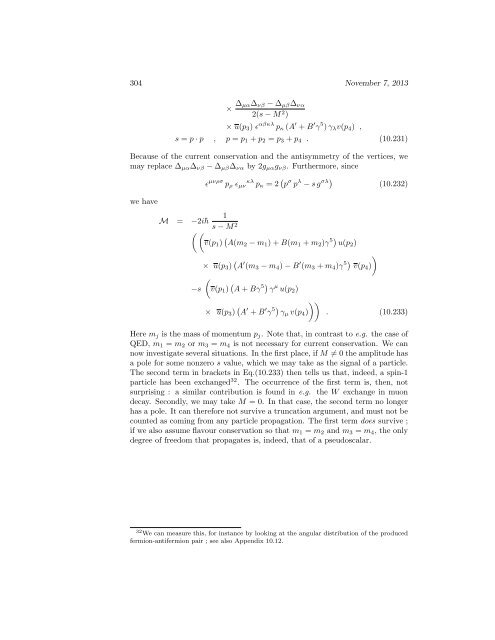
- Page 302 and 303: 302 November 7, 2013 our candidate
- Page 306 and 307: 306 November 7, 2013 where m and m
- Page 308 and 309: 308 November 7, 2013 cross section
- Page 310 and 311: 310 November 7, 2013 As we can see,
- Page 312 and 313: 312 November 7, 2013 which may help
- Page 314 and 315: 314 November 7, 2013 Let now form t
- Page 316: 316 November 7, 2013 and by inspect