Predictive Control of Three Phase AC/DC Converters

44 CHAPTER 4. PREDICTIVE DIRECT POWER CONTROL
(a)
(b)
0
∆ P 0
∆ P 7
∆ P 6
∆ P 1
∆ P 2 ∆ P 3
∆ P 4
∆ P 5
0
∆ Q 7
∆ Q 0
∆ Q 4
∆ Q 5
∆ Q 6
∆ Q 1
∆ Q 2
∆ Q 3
0 0.002 0.004 0.006 0.008 0.01 0.012 0.014 0.016 0.018 0.02
0 0.002 0.004 0.006 0.008 0.01 0.012 0.014 0.016 0.018 0.02
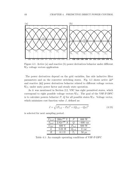
Figure 4.1: Active (a) and reactive (b) power derivatives behavior under different
U P voltage vectors application
The power derivatives depend on the grid variables, line side inductive filter
parameters and on the converter switching states. Fig. 4.1 shows active ∆P
and reactive ∆Q power derivatives behavior related to different voltage vectors
U P , under unity power factor and steady state operation.
As it was mentioned in Section 2.2, VSC has eight permitted states, which
correspond to eight possible voltage vectors U P . The goal of the VSF-P-DPC
is to calculate powers behavior P , Q for all possible states U P . Voltage vector,
which minimizes cost function value J, defined as:
√
J = (P ref − P P ) 2 + (Q ref − Q P ) 2 (4.15)
is selected for next sampling period.
U Lαβ 200e j45 V P 600 W
I Lαβ 2.82e j90 A Q −600 var
U DC 600 V P ref 600 W
L 0.01 H Q ref 0 var
R 0.1 Ω T s 50 µs
Table 4.1: An example operating conditions of VSF-P-DPC