link to my thesis

96 CHAPTER 6. ITERATIVE EIGENVALUE SOLVERS
A second approach for Stetter projection, which works for negative values as well
as for complex values in the approximate eigenvector, is described next. The idea is
to compare the structured eigenvector v and the multiplication ṽ of the eigenvector
with a variable x i : ṽ = x i v. Then the vectors ṽ and v have entries in common which
describe the relations between the separate entries in v itself. If an approximate vector
is indeed a ‘true’ eigenvector, then the values within the eigenvector should satisfy
these relations too. The relations can be expressed in the form of P (x 1 ,...,x n ) T −u =
0 for all the variables x i . A linear least-squares method can compute the solution
(x 1 ,...,x n ) T with the smallest error e = P (x 1 ,...,x n ) T − u. This approach is
illustrated with an example.
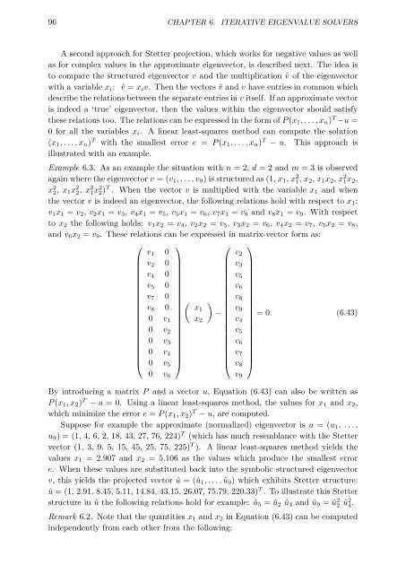
Example 6.3. As an example the situation with n =2,d = 2 and m = 3 is observed
again where the eigenvector v =(v 1 ,...,v 9 ) is structured as (1, x 1 ,x 2 1,x 2 ,x 1 x 2 ,x 2 1x 2 ,
x 2 2,x 1 x 2 2,x 2 1x 2 2) T . When the vector v is multiplied with the variable x 1 and when
the vector v is indeed an eigenvector, the following relations hold with respect to x 1 :
v 1 x 1 = v 2 , v 2 x 1 = v 3 , v 4 x 1 = v 5 , v 5 x 1 = v 6 , v 7 x 1 = v 8 and v 8 x 1 = v 9 . With respect
to x 2 the following holds: v 1 x 2 = v 4 , v 2 x 2 = v 5 , v 3 x 2 = v 6 , v 4 x 2 = v 7 , v 5 x 2 = v 8 ,
and v 6 x 2 = v 9 . These relations can be expressed in matrix-vector form as:
⎛
⎜
⎝
⎞
v 1 0
v 2 0
v 4 0
v 5 0
v 7 0
v 8 0
0 v 1
0 v 2
0 v 3
0 v 4
⎟
0 v 5
⎠
0 v 6
(
x1
x 2
)
⎛
−
⎜
⎝
v 2
v 3
v 5
v 6
v 8
v 9
v 4
v 5
v 6
v 7
v 8
v 9
⎞
=0. (6.43)
⎟
⎠
By introducing a matrix P and a vector u, Equation (6.43) can also be written as
P (x 1 ,x 2 ) T − u = 0. Using a linear least-squares method, the values for x 1 and x 2 ,
which minimize the error e = P (x 1 ,x 2 ) T − u, are computed.
Suppose for example the approximate (normalized) eigenvector is u =(u 1 , ...,
u 9 )=(1, 4, 6, 2, 18, 43, 27, 76, 224) T (which has much resemblance with the Stetter
vector (1, 3, 9, 5, 15, 45, 25, 75, 225) T ). A linear least-squares method yields the
values x 1 =2.907 and x 2 =5.106 as the values which produce the smallest error
e. When these values are substituted back into the symbolic structured eigenvector
v, this yields the projected vector û =(û 1 ,...,û 9 ) which exhibits Stetter structure:
û =(1, 2.91, 8.45, 5.11, 14.84, 43.15, 26.07, 75.79, 220.33) T . To illustrate this Stetter
structure in û the following relations hold for example: û 5 =û 2 û 4 and û 9 =û 2 2 û 2 4.
Remark 6.2. Note that the quantities x 1 and x 2 in Equation (6.43) can be computed
independently from each other from the following: