link to my thesis

11.5. EXAMPLE 223
AãN−2 (ρ 1 ,ρ 2 ) T are constructed. The monomial basis B used for constructing these
matrices is:
B = {1,x 1 ,x 2 ,x 1 x 2 ,x 3 ,x 1 x 3 ,x 2 x 3 ,x 1 x 2 x 3 ,x 4 ,x 1 x 4 ,x 2 x 4 ,
x 1 x 2 x 4 ,x 3 x 4 ,x 1 x 3 x 4 ,x 2 x 3 x 4 ,x 1 x 2 x 3 x 4 }.
(11.80)
After making the matrices AãN−1 (ρ 1 ,ρ 2 ) T and AãN−2 (ρ 1 ,ρ 2 ) T polynomial in (ρ 1 ,ρ 2 )
(see Theorem 10.1), they are denoted by Ãã N−1
(ρ 1 ,ρ 2 ) T and Ãã N−2
(ρ 1 ,ρ 2 ) T . The
dimensions of these matrices are 2 4 ×2 4 =16×16 and the total degree of all the terms
is N − 1 = 3 (analogous to the result in Corollary 10.2). The trivial/zero solution
can be split off from the matrices immediately by removing the first column, which is
a zero column, and the first row of both the matrices. This brings the dimensions of
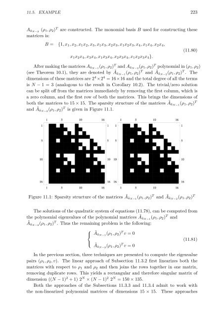
both the matrices to 15 × 15. The sparsity structure of the matrices Ãã N−1
(ρ 1 ,ρ 2 ) T
and Ãã N−2
(ρ 1 ,ρ 2 ) T is given in Figure 11.1.
Figure 11.1: Sparsity structure of the matrices Ãã N−1
(ρ 1 ,ρ 2 ) T and Ãã N−2
(ρ 1 ,ρ 2 ) T
The solutions of the quadratic system of equations (11.78), can be computed from
the polynomial eigenvalues of the polynomial matrices Ãã N−1
(ρ 1 ,ρ 2 ) T and
ÃãN−2 (ρ 1 ,ρ 2 ) T . Thus the remaining problem is the following:
⎧
⎨
⎩
ÃãN−1 (ρ 1 ,ρ 2 ) T v =0
ÃãN−2 (ρ 1 ,ρ 2 ) T v =0
(11.81)
In the previous section, three techniques are presented to compute the eigenvalue
pairs (ρ 1 ,ρ 2 ,v). The linear approach of Subsection 11.3.2 first linearizes both the
matrices with respect to ρ 1 and ρ 2 and then joins the rows together in one matrix,
removing duplicate rows. This yields a rectangular and therefore singular matrix of
dimension ((N − 1) 2 +1)2 N × (N − 1) 2 2 N = 150 × 135.
Both the approaches of the Subsections 11.3.3 and 11.3.4 admit to work with
the non-linearized polynomial matrices of dimensions 15 × 15. These approaches