link to my thesis

162 CHAPTER 10. H 2 MODEL-ORDER REDUCTION FROM ORDER N TO N-2
which satisfy the linear constraint in (10.3).
Till now we have treated the general case where q 0 0 in (8.20). If q 0 = 0 we end
up in a slightly different situation which can be treated as follows. If q 0 = 0, then
the polynomial q(s) in (8.19) equals q 1 s. This allows one to rewrite Equation (8.18)
into the form:
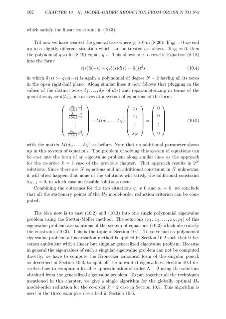
e(s)ã(−s) − q 1 b(s)d(s) =ã(s) 2 s (10.4)
in which ã(s) :=q 1 a(−s) is again a polynomial of degree N − 2 having all its zeros
in the open right-half plane. Along similar lines it now follows that plugging in the
values of the distinct zeros δ 1 ,...,δ N of d(s) and reparameterizing in terms of the
quantities x i := ã(δ i ), one arrives at a system of equations of the form:
⎛
δ 1
⎞
⎛ ⎞ ⎛ ⎞
e(δ 1) x2 1
x 1 0
δ 2
e(δ 2) x2 2
x 2
0
⎜
− M(δ ⎝ . ⎟ 1 ,...,δ N )
⎜
=
⎠
⎝ .
⎟ ⎜
(10.5)
⎠ ⎝ .
⎟
⎠
0
δ N
e(δ N ) x2 N
with the matrix M(δ 1 ,..., δ N ) as before. Note that no additional parameter shows
up in this system of equations. The problem of solving this system of equations can
be cast into the form of an eigenvalue problem along similar lines as the approach
for the co-order k = 1 case of the previous chapter. That approach results in 2 N
solutions. Since there are N equations and an additional constraint in N unknowns,
it will often happen that none of the solutions will satisfy the additional constraint
ã N−1 = 0, in which case no feasible solutions occur.
Combining the outcomes for the two situations q 0 0 and q 0 = 0, we conclude
that all the stationary points of the H 2 model-order reduction criterion can be computed.
The idea now is to cast (10.2) and (10.3) into one single polynomial eigenvalue
problem using the Stetter-Möller method. The solutions (x 1 ,x 2 ,...,x N ,ρ 1 ) of this
eigenvalue problem are solutions of the system of equations (10.2) which also satisfy
the constraint (10.3). This is the topic of Section 10.1. To solve such a polynomial
eigenvalue problem a linearization method is applied in Section 10.2 such that it becomes
equivalent with a linear but singular generalized eigenvalue problem. Because
in general the eigenvalues of such a singular eigenvalue problem can not be computed
directly, we have to compute the Kronecker canonical form of the singular pencil,
as described in Section 10.3, to split off the unwanted eigenvalues. Section 10.4 describes
how to compute a feasible approximation of order N − 2 using the solutions
obtained from the generalized eigenvalue problem. To put together all the techniques
mentioned in this chapter, we give a single algorithm for the globally optimal H 2
model-order reduction for the co-order k = 2 case in Section 10.5. This algorithm is
used in the three examples described in Section 10.6.
x N