link to my thesis

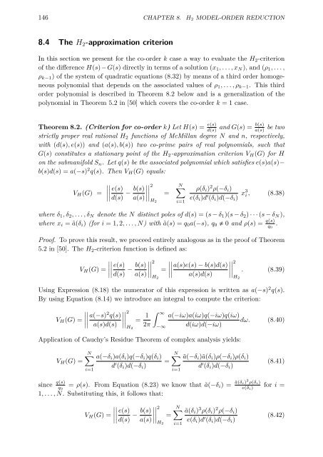
146 CHAPTER 8. H 2 MODEL-ORDER REDUCTION
8.4 The H 2 -approximation criterion
In this section we present for the co-order k case a way to evaluate the H 2 -criterion
of the difference H(s)−G(s) directly in terms of a solution (x 1 ,...,x N ), and (ρ 1 ,...,
ρ k−1 ) of the system of quadratic equations (8.32) by means of a third order homogeneous
polynomial that depends on the associated values of ρ 1 ,...,ρ k−1 . This third
order polynomial is described in Theorem 8.2 below and is a generalization of the
polynomial in Theorem 5.2 in [50] which covers the co-order k = 1 case.
Theorem 8.2. (Criterion for co-order k) Let H(s) = e(s)
d(s)
b(s)
and G(s) =
a(s)
be two
strictly proper real rational H 2 functions of McMillan degree N and n, respectively,
with (d(s),e(s)) and (a(s),b(s)) two co-prime pairs of real polynomials, such that
G(s) constitutes a stationary point of the H 2 -approximation criterion V H (G) for H
on the submanifold S n .Letq(s) be the associated polynomial which satisfies e(s)a(s)−
b(s)d(s) =a(−s) 2 q(s). Then V H (G) equals:
V H (G) =
e(s)
∣∣d(s) − b(s)
a(s) ∣∣
2
H 2
=
N∑
i=1
ρ(δ i ) 2 ρ(−δ i )
e(δ i )d ′ (δ i )d(−δ i ) x3 i , (8.38)
where δ 1 ,δ 2 ,...,δ N denote the N distinct poles of d(s) =(s − δ 1 )(s − δ 2 ) ···(s − δ N ),
where x i =ã(δ i ) (for i =1, 2,...,N) with ã(s) =q 0 a(−s), q 0 0 and ρ(s) = q(s)
q 0
.
Proof. To prove this result, we proceed entirely analogous as in the proof of Theorem
5.2 in [50]. The H 2 -criterion function is defined as:
V H (G) =
e(s)
∣∣d(s) − b(s)
a(s) ∣∣
2
H 2
=
2
a(s)e(s) − b(s)d(s)
∣∣
a(s)d(s) ∣∣
. (8.39)
H 2
Using Expression (8.18) the numerator of this expression is written as a(−s) 2 q(s).
By using Equation (8.14) we introduce an integral to compute the criterion:
V H (G) =
a(−s) 2 2
q(s)
∣∣
a(s)d(s) ∣∣
= 1 ∫ ∞
a(−iω)a(iω)q(−iω)q(iω)
dω. (8.40)
H 2
2π −∞ d(iω)d(−iω)
Application of Cauchy’s Residue Theorem of complex analysis yields:
V H (G) =
N∑
i=1
a(−δ i )a(δ i )q(−δ i )q(δ i )
d ′ (δ i )d(−δ i )
=
N∑
i=1
ã(−δ i )ã(δ i )ρ(−δ i )ρ(δ i )
d ′ (δ i )d(−δ i )
(8.41)
since q(s)
q 0
= ρ(s). From Equation (8.23) we know that ã(−δ i )= ã(δi)2 ρ(δ i)
e(δ i)
for i =
1,...,N. Substituting this, it follows that:
V H (G) =
e(s)
∣∣d(s) − b(s)
a(s) ∣∣
2
H 2
=
N∑
i=1
ã(δ i ) 3 ρ(δ i ) 2 ρ(−δ i )
e(δ i )d ′ (δ i )d(−δ i )
(8.42)