- Page 3 and 4:
Stellingen behorende bij het proefs
- Page 5 and 6:
ALGEBRAIC POLYNOMIAL SYSTEM SOLVING
- Page 7 and 8:
ALGEBRAIC POLYNOMIAL SYSTEM SOLVING
- Page 9:
For all those I love...
- Page 12 and 13:
ii CONTENTS II Global Optimization
- Page 14 and 15:
iv CONTENTS 12.2 Directions for fur
- Page 17 and 18:
Chapter 1 Introduction 1.1 Motivati
- Page 19 and 20:
1.3. RESEARCH QUESTIONS 5 The goal
- Page 21 and 22:
1.4. THESIS OUTLINE 7 Jacobi-Davids
- Page 23:
Part I General introduction and bac
- Page 26 and 27:
12 CHAPTER 2. ALGEBRAIC BACKGROUND
- Page 28 and 29:
14 CHAPTER 2. ALGEBRAIC BACKGROUND
- Page 30 and 31:
16 CHAPTER 2. ALGEBRAIC BACKGROUND
- Page 32 and 33:
18 CHAPTER 2. ALGEBRAIC BACKGROUND
- Page 34 and 35:
20 CHAPTER 2. ALGEBRAIC BACKGROUND
- Page 36 and 37:
22 CHAPTER 2. ALGEBRAIC BACKGROUND
- Page 39 and 40:
Chapter 3 Solving polynomial system
- Page 41 and 42:
3.1. SOLVING POLYNOMIAL EQUATIONS I
- Page 43 and 44:
3.2. METHODS FOR SOLVING POLYNOMIAL
- Page 45 and 46:
3.2. METHODS FOR SOLVING POLYNOMIAL
- Page 47 and 48:
3.2. METHODS FOR SOLVING POLYNOMIAL
- Page 49 and 50:
3.3. THE STETTER-MÖLLER MATRIX MET
- Page 51 and 52:
3.5. EXAMPLE 37 applying the Stette
- Page 53:
3.5. EXAMPLE 39 be: I = 〈13x 2 2
- Page 57 and 58:
Chapter 4 Global optimization of mu
- Page 59 and 60:
4.1. THE GLOBAL MINIMUM OF A DOMINA
- Page 61 and 62:
4.3. AN EXAMPLE 47 Using the matric
- Page 63 and 64:
4.3. AN EXAMPLE 49 the Stetter-Möl
- Page 65 and 66:
Chapter 5 An nD-systems approach in
- Page 67 and 68:
5.1. THE ND-SYSTEM 53 cerned with t
- Page 69 and 70:
5.1. THE ND-SYSTEM 55 Example 5.1.
- Page 71 and 72:
5.1. THE ND-SYSTEM 57 Figure 5.2: T
- Page 73 and 74:
5.3. EFFICIENCY OF THE ND-SYSTEMS A
- Page 75 and 76:
5.3. EFFICIENCY OF THE ND-SYSTEMS A
- Page 77 and 78:
5.3. EFFICIENCY OF THE ND-SYSTEMS A
- Page 79 and 80:
5.3. EFFICIENCY OF THE ND-SYSTEMS A
- Page 81 and 82:
5.3. EFFICIENCY OF THE ND-SYSTEMS A
- Page 83 and 84:
5.3. EFFICIENCY OF THE ND-SYSTEMS A
- Page 85 and 86:
5.3. EFFICIENCY OF THE ND-SYSTEMS A
- Page 87 and 88:
5.3. EFFICIENCY OF THE ND-SYSTEMS A
- Page 89 and 90:
5.3. EFFICIENCY OF THE ND-SYSTEMS A
- Page 91 and 92:
5.3. EFFICIENCY OF THE ND-SYSTEMS A
- Page 93 and 94:
5.3. EFFICIENCY OF THE ND-SYSTEMS A
- Page 95 and 96:
Chapter 6 Iterative eigenvalue solv
- Page 97 and 98:
6.2. THE JACOBI-DAVIDSON METHOD 83
- Page 99 and 100:
6.2. THE JACOBI-DAVIDSON METHOD 85
- Page 101 and 102:
6.4. PROJECTION TO STETTER-STRUCTUR
- Page 103 and 104:
6.4. PROJECTION TO STETTER-STRUCTUR
- Page 105 and 106:
6.4. PROJECTION TO STETTER-STRUCTUR
- Page 107 and 108:
6.4. PROJECTION TO STETTER-STRUCTUR
- Page 109 and 110:
6.4. PROJECTION TO STETTER-STRUCTUR
- Page 111 and 112:
6.4. PROJECTION TO STETTER-STRUCTUR
- Page 113 and 114:
6.4. PROJECTION TO STETTER-STRUCTUR
- Page 115 and 116:
6.4. PROJECTION TO STETTER-STRUCTUR
- Page 117 and 118:
6.5. A JACOBI-DAVIDSON METHOD FOR C
- Page 119:
6.5. A JACOBI-DAVIDSON METHOD FOR C
- Page 122 and 123:
108 CHAPTER 7. NUMERICAL EXPERIMENT
- Page 124 and 125:
110 CHAPTER 7. NUMERICAL EXPERIMENT
- Page 126 and 127:
112 CHAPTER 7. NUMERICAL EXPERIMENT
- Page 128 and 129:
114 CHAPTER 7. NUMERICAL EXPERIMENT
- Page 130 and 131:
116 CHAPTER 7. NUMERICAL EXPERIMENT
- Page 132 and 133:
118 CHAPTER 7. NUMERICAL EXPERIMENT
- Page 134 and 135:
120 CHAPTER 7. NUMERICAL EXPERIMENT
- Page 136 and 137:
122 CHAPTER 7. NUMERICAL EXPERIMENT
- Page 138 and 139:
124 CHAPTER 7. NUMERICAL EXPERIMENT
- Page 140 and 141:
126 CHAPTER 7. NUMERICAL EXPERIMENT
- Page 142 and 143:
128 CHAPTER 7. NUMERICAL EXPERIMENT
- Page 145:
Part III H 2 Model-order Reduction
- Page 148 and 149:
134 CHAPTER 7. NUMERICAL EXPERIMENT
- Page 150 and 151:
136 CHAPTER 8. H 2 MODEL-ORDER REDU
- Page 152 and 153:
138 CHAPTER 8. H 2 MODEL-ORDER REDU
- Page 154 and 155:
140 CHAPTER 8. H 2 MODEL-ORDER REDU
- Page 156 and 157:
142 CHAPTER 8. H 2 MODEL-ORDER REDU
- Page 158 and 159:
144 CHAPTER 8. H 2 MODEL-ORDER REDU
- Page 160 and 161:
146 CHAPTER 8. H 2 MODEL-ORDER REDU
- Page 162 and 163:
148 CHAPTER 8. H 2 MODEL-ORDER REDU
- Page 164 and 165:
150 CHAPTER 8. H 2 MODEL-ORDER REDU
- Page 166 and 167:
152 CHAPTER 9. H 2 MODEL-ORDER REDU
- Page 168 and 169:
154 CHAPTER 9. H 2 MODEL-ORDER REDU
- Page 170 and 171:
156 CHAPTER 9. H 2 MODEL-ORDER REDU
- Page 172 and 173:
158 CHAPTER 9. H 2 MODEL-ORDER REDU
- Page 175 and 176:
Chapter 10 H 2 Model-order reductio
- Page 177 and 178:
10.1. SOLVING THE SYSTEM OF QUADRAT
- Page 179 and 180:
10.1. SOLVING THE SYSTEM OF QUADRAT
- Page 181 and 182:
10.2. LINEARIZING A POLYNOMIAL EIGE
- Page 183 and 184:
10.3. THE KRONECKER CANONICAL FORM
- Page 185 and 186:
10.3. THE KRONECKER CANONICAL FORM
- Page 187 and 188:
10.3. THE KRONECKER CANONICAL FORM
- Page 189 and 190:
10.3. THE KRONECKER CANONICAL FORM
- Page 191 and 192:
10.3. THE KRONECKER CANONICAL FORM
- Page 193 and 194:
10.4. COMPUTING THE APPROXIMATION G
- Page 195 and 196:
10.6. EXAMPLES 181 5. Compute the n
- Page 197 and 198:
10.6. EXAMPLES 183 Figure 10.1: Spa
- Page 199 and 200:
10.6. EXAMPLES 185 Figure 10.3: The
- Page 201 and 202:
10.6. EXAMPLES 187 Figure 10.5: Imp
- Page 203 and 204:
10.6. EXAMPLES 189 Figure 10.7: Str
- Page 205 and 206:
10.6. EXAMPLES 191 Figure 10.8: Pol
- Page 207 and 208:
10.6. EXAMPLES 193 Table 10.1: Redu
- Page 209 and 210:
Chapter 11 H 2 Model-order reductio
- Page 211 and 212:
11.2. LINEARIZING THE TWO-PARAMETER
- Page 213 and 214: 11.3. KRONECKER CANONICAL FORM OF A
- Page 215 and 216: 11.3. KRONECKER CANONICAL FORM OF A
- Page 217 and 218: 11.3. KRONECKER CANONICAL FORM OF A
- Page 219 and 220: 11.3. KRONECKER CANONICAL FORM OF A
- Page 221 and 222: 11.3. KRONECKER CANONICAL FORM OF A
- Page 223 and 224: 11.3. KRONECKER CANONICAL FORM OF A
- Page 225 and 226: 11.3. KRONECKER CANONICAL FORM OF A
- Page 227 and 228: 11.3. KRONECKER CANONICAL FORM OF A
- Page 229 and 230: 11.3. KRONECKER CANONICAL FORM OF A
- Page 231 and 232: 11.3. KRONECKER CANONICAL FORM OF A
- Page 233 and 234: 11.3. KRONECKER CANONICAL FORM OF A
- Page 235 and 236: 11.4. COMPUTING THE APPROXIMATION G
- Page 237 and 238: 11.5. EXAMPLE 223 AãN−2 (ρ 1 ,
- Page 239 and 240: 11.5. EXAMPLE 225 of both matrices
- Page 241 and 242: 11.5. EXAMPLE 227 of solutions (ρ
- Page 243 and 244: Chapter 12 Conclusions & directions
- Page 245 and 246: 12.1. CONCLUSIONS 231 used first. T
- Page 247 and 248: 12.1. CONCLUSIONS 233 solver as des
- Page 249 and 250: 12.2. DIRECTIONS FOR FURTHER RESEAR
- Page 251 and 252: Bibliography [1] W. Adams and P. Lo
- Page 253 and 254: BIBLIOGRAPHY 239 [26] A. Cayley. On
- Page 255 and 256: BIBLIOGRAPHY 241 [58] M.E. Hochsten
- Page 257: BIBLIOGRAPHY 243 [90] S. Prajna, A.
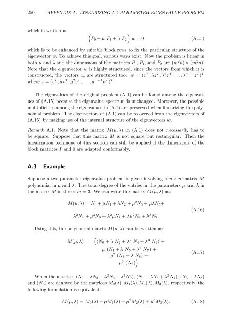
- Page 261 and 262: Appendix A A linearization techniqu
- Page 263: A.2. LINEARIZATION WITH RESPECT TO
- Page 267: A.3. EXAMPLE 253 where the eigenvec
- Page 270 and 271: 256 APPENDIX B. POLYNOMIAL TEST SET
- Page 272 and 273: 258 SUMMARY vector. This routine is
- Page 274 and 275: 260 SUMMARY globally optimal approx
- Page 276 and 277: 262 SAMENVATTING De matrix-vrije im
- Page 278 and 279: 264 SAMENVATTING eigenwaarde proble
- Page 281 and 282: List of Publications [1] I.W.M. Ble
- Page 283 and 284: List of Symbols and Abbreviations A
- Page 285 and 286: LIST OF FIGURES 271 7.7 Residual no
- Page 287 and 288: Index H 2 model-order reduction pro


