Introductory Physics Volume Two

6.2 Faraday’s Law 117
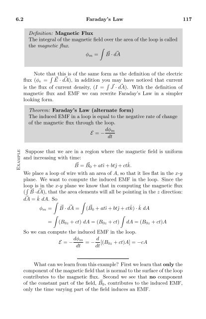
Definition: Magnetic Flux
The integral of the magnetic field over the area of the loop is called
the magnetic flux.
∫
φ m = ⃗B · dA ⃗
Note that this is of the same form as the definition of the electric
flux (φ e = ∫ E ⃗ · dA), ⃗ in addition you may have noticed that current
is the flux of current density, (I = ∫ J ⃗ · dA). ⃗ With the definition of
magnetic flux and EMF we can rewrite Faraday’s Law in a simpler
looking form.
Theorem: Faraday’s Law (alternate form)
The induced EMF in a loop is equal to the negative rate of change
of the magnetic flux through the loop.
E = − dφ m
dt
Example
Suppose that we are in a region where the magnetic field is uniform
and increasing with time:
⃗B = ⃗ B 0 + atî + btĵ + ctˆk.
We place a loop of wire with an area of A, so that it lies flat in the x-y
plane. We want to compute the induced EMF in the loop. Since the
loop is in the x-y plane we know that in computing the magnetic flux
( ∫ B ⃗ · dA), ⃗ that the area elements will all be pointing in the z direction:
dA ⃗ = ˆk dA. So ∫ ∫
φ m = ⃗B · dA ⃗ = ( B ⃗ 0 + atî + btĵ + ctˆk) · ˆk dA
∫
∫
= (B 0z + ct) dA = (B 0z + ct) dA = (B 0z + ct)A
So we can compute the induced EMF in the loop.
E = − dφ m
dt
= − d dt [(B 0z + ct)A] = −cA
What can we learn from this example? First we learn that only the
component of the magnetic field that is normal to the surface of the loop
contributes to the magnetic flux. Second we see that no component
of the constant part of the field, ⃗ B 0 , contributes to the induced EMF,
only the time varying part of the field induces an EMF.