Introductory Physics Volume Two

5.1 Sources of Magnetic Field 99
⊲ Problem 5.2
Write a parameterization for a parabola that goes through the three
points (-1,0), (0,1) and (1,0).
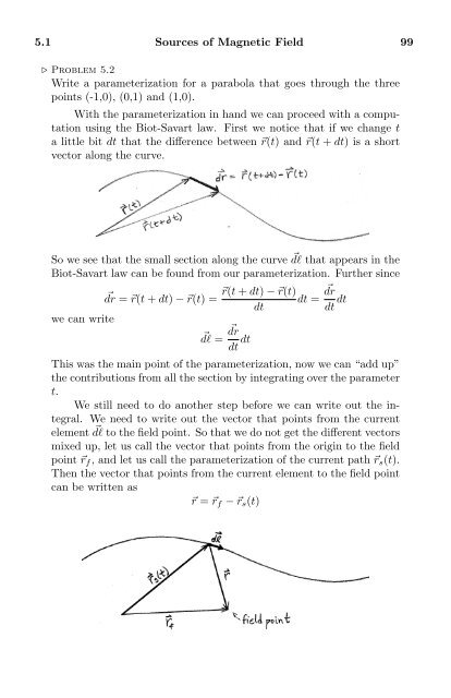
With the parameterization in hand we can proceed with a computation
using the Biot-Savart law. First we notice that if we change t
a little bit dt that the difference between ⃗r(t) and ⃗r(t + dt) is a short
vector along the curve.
So we see that the small section along the curve ⃗ dl that appears in the
Biot-Savart law can be found from our parameterization. Further since
we can write
⃗dr = ⃗r(t + dt) − ⃗r(t) =
⃗r(t + dt) − ⃗r(t) dr
dt = ⃗ dt
dt dt
⃗dl = ⃗ dr
dt dt
This was the main point of the parameterization, now we can “add up”
the contributions from all the section by integrating over the parameter
t.
We still need to do another step before we can write out the integral.
We need to write out the vector that points from the current
element ⃗ dl to the field point. So that we do not get the different vectors
mixed up, let us call the vector that points from the origin to the field
point ⃗r f , and let us call the parameterization of the current path ⃗r s (t).
Then the vector that points from the current element to the field point
can be written as
⃗r = ⃗r f − ⃗r s (t)