Introductory Physics Volume Two

98 Sources of Magnetic Field 5.1
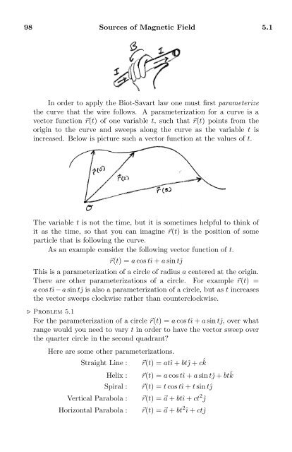
In order to apply the Biot-Savart law one must first parameterize
the curve that the wire follows. A parameterization for a curve is a
vector function ⃗r(t) of one variable t, such that ⃗r(t) points from the
origin to the curve and sweeps along the curve as the variable t is
increased. Below is picture such a vector function at the values of t.
The variable t is not the time, but it is sometimes helpful to think of
it as the time, so that you can imagine ⃗r(t) is the position of some
particle that is following the curve.
As an example consider the following vector function of t.
⃗r(t) = a cos tî + a sin tĵ
This is a parameterization of a circle of radius a centered at the origin.
There are other parameterizations of a circle. For example ⃗r(t) =
a cos tî − a sin tĵ is also a parameterization of a circle, but as t increases
the vector sweeps clockwise rather than counterclockwise.
⊲ Problem 5.1
For the parameterization of a circle ⃗r(t) = a cos tî + a sin tĵ, over what
range would you need to vary t in order to have the vector sweep over
the quarter circle in the second quadrant?
Here are some other parameterizations.
Straight Line :
Helix :
Spiral :
Vertical Parabola :
Horizontal Parabola :
⃗r(t) = atî + btĵ + cˆk
⃗r(t) = a cos tî + a sin tĵ + btˆk
⃗r(t) = t cos tî + t sin tĵ
⃗r(t) = ⃗a + btî + ct 2 ĵ
⃗r(t) = ⃗a + bt 2 î + ctĵ