- Page 1 and 2: 1 Introductory Physics Volume Two S
- Page 3 and 4: 1.1 Electric Charge 3 Demo 1 Electr
- Page 5 and 6: 1.1 Electric Charge 5 Then charge a
- Page 7 and 8: - - - - - 1.2 Coulomb’s Law 7 How
- Page 9 and 10: 1.2 Coulomb’s Law 9 Example Consi
- Page 11 and 12: 1.3 Electric Field 11 + - Compute t
- Page 13 and 14: 1.3 Electric Field 13 points a well
- Page 15 and 16: 1.3 Electric Field 15 Look back now
- Page 17 and 18: 1.5 Continuous Charge Distributions
- Page 19 and 20: 1.6 Gauss’s Law 19 § 1.6 Gauss
- Page 21 and 22: 1.6 Gauss’s Law 21 Suppose that y
- Page 23 and 24: 1.7 More Examples 23 ⊲ Problem 1.
- Page 25 and 26: 1.7 More Examples 25 The net force
- Page 27 and 28: 1.7 More Examples 27 out the net fo
- Page 29 and 30: 1.7 More Examples 29 -4q +2q -q E -
- Page 31 and 32: 1.7 More Examples 31 The area vecto
- Page 33 and 34: 1.8 Homework 33 ⊲ Problem 1.14 Ri
- Page 35 and 36: 1.9 Summary 35 § 1.9 Summary Defin
- Page 37 and 38: 2.1 Electric Potential 37 2 Electri
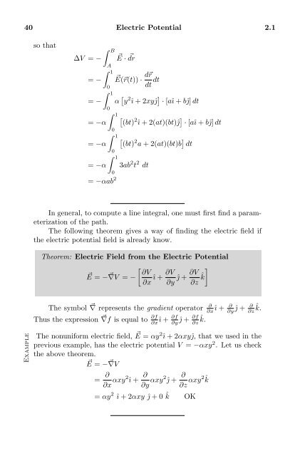
- Page 39: 2.1 Electric Potential 39 Example S
- Page 43 and 44: 2.3 Conductors in Equilibrium 43
- Page 45 and 46: 2.4 Capacitors 45 § 2.4 Capacitors
- Page 47 and 48: 2.5 Energy in an Electric Field 47
- Page 49 and 50: 2.7 More Examples 49 ⊲ Problem 2.
- Page 51 and 52: 2.7 More Examples 51 The resulting
- Page 53 and 54: 2.8 Homework 53 add up potential du
- Page 55 and 56: 2.8 Homework 55 ⊲ Problem 2.27 Ho
- Page 57 and 58: 3.2 Electric Current 57 3 Circuits
- Page 59 and 60: 3.3 Ohm’s Law 59 Some materials,
- Page 61 and 62: 3.5 Kirchhoff’s Rules 61 ⊲ Prob
- Page 63 and 64: 3.6 Resistors in Combination 63 par
- Page 65 and 66: 3.8 Capacitor Circuits 65 Theorem:
- Page 67 and 68: 3.9 More Examples 67 Note that the
- Page 69 and 70: 3.9 More Examples 69 This mean that
- Page 71 and 72: 3.9 More Examples 71 15Ω 5Ω 10Ω
- Page 73 and 74: 3.9 More Examples 73 First combine
- Page 75 and 76: 3.10 Homework 75 ⊲ Problem 3.16 B
- Page 77 and 78: 3.10 Homework 77 4 µF + - 2 µF +
- Page 79 and 80: 3.11 Summary 79 § 3.11 Summary Def
- Page 81 and 82: 4.2 Magnetic Force on a Current 81
- Page 83 and 84: 4.3 Trajectories Under Magnetic For
- Page 85 and 86: 4.4 Lorentz Force 85 with a charge
- Page 87 and 88: 4.5 Hall Effect 87 But this charge
- Page 89 and 90: 4.6 More Examples 89 -e F E v F B =
- Page 91 and 92:
4.6 More Examples 91 The force on t
- Page 93 and 94:
4.7 Homework 93 Imagine the closed
- Page 95 and 96:
4.7 Homework 95 circular orbits. Wr
- Page 97 and 98:
5.1 Sources of Magnetic Field 97 5
- Page 99 and 100:
5.1 Sources of Magnetic Field 99
- Page 101 and 102:
5.2 Ampere’s Law 101 and ⃗ dr s
- Page 103 and 104:
5.2 Ampere’s Law 103 This satisfi
- Page 105 and 106:
5.4 More Examples 105 distance r fr
- Page 107 and 108:
5.4 More Examples 107 up the integr
- Page 109 and 110:
5.4 More Examples 109 Use the Biot-
- Page 111 and 112:
5.5 Homework 111 The magnetic force
- Page 113 and 114:
5.5 Homework 113 3.00 A 1.00 A 1 mm
- Page 115 and 116:
6.2 Faraday’s Law 115 6 Time Vary
- Page 117 and 118:
6.2 Faraday’s Law 117 Definition:
- Page 119 and 120:
6.3 Maxwell’s Extension of Ampere
- Page 121 and 122:
6.4 Inductance 121 Example Suppose
- Page 123 and 124:
6.7 AC Circuit Elements 123 + V S-
- Page 125 and 126:
6.8 Phasor Diagrams 125 Theorem: Im
- Page 127 and 128:
6.8 Phasor Diagrams 127 What we wan
- Page 129 and 130:
6.9 Homework 129 ⊲ Problem 6.6 Sh
- Page 131 and 132:
6.9 Homework 131 (b) A small circul
- Page 133 and 134:
6.9 Homework 133 maximum current in
- Page 135 and 136:
6.10 Summary 135 § 6.10 Summary De
- Page 137 and 138:
7.1 Maxwell Equations 137 7 Wave Op
- Page 139 and 140:
7.2 Describing Oscillations 139 tio
- Page 141 and 142:
7.3 Describing Waves 141 For a harm
- Page 143 and 144:
7.3 Describing Waves 143 Definition
- Page 145 and 146:
7.4 Electromagnetic Waves 145 § 7.
- Page 147 and 148:
7.5 Interference of Waves 147 I I A
- Page 149 and 150:
7.7 Interference of Two Sources 149
- Page 151 and 152:
7.8 Far Field Approximation 151 §
- Page 153 and 154:
7.9 Thin Film Interference 153 pass
- Page 155 and 156:
7.11 Homework 155 Second Min First
- Page 157 and 158:
7.11 Homework 157 θ 2 d θ 1 θ 2
- Page 159 and 160:
7.12 Summary 159 § 7.12 Summary De
- Page 161 and 162:
8.2 Reflection 161 8 Geometric Opti
- Page 163 and 164:
8.4 Snell’s Law 163 We see then t
- Page 165 and 166:
8.5 Virtual Image Caused by Refract
- Page 167 and 168:
8.6 Thin Lens Equation 167 back in
- Page 169 and 170:
8.7 Virtual Image in a Converging L
- Page 171 and 172:
8.8 Diverging Lenses 171 (b) virtua
- Page 173 and 174:
8.10 Multi-Lens Optical Systems 173
- Page 175 and 176:
8.11 Homework 175 We can also compu
- Page 177 and 178:
@ Summary 177 § 8.12 Summary Facts
- Page 179 and 180:
A Hints 179 1.14 Since this is only
- Page 181 and 182:
A Hints 181 2.27 Imagine that you b
- Page 183 and 184:
A Hints 183 4.12 Consider the vecto
- Page 185 and 186:
A Hints 185 7.26 The distance from
- Page 187 and 188:
B Index 187 † Ohm’s Law: Resist
- Page 189 and 190:
B Index 189
- Page 191 and 192:
C Power Series Expansions 191 The F
- Page 193:
D Unit Prefixes 193 § D.3 Fundamen