Woo Young Lee Lecture Notes on Operator Theory

CHAPTER 4.
WEIGHTED SHIFTS
are both positive
( [
k =
] [
m+1
2
, l =
⎡ ⎤
γ k+1
⎢
⎣
⎥
. ⎦
γ 2k+1
] )
m
2
+ 1 and the vector
⎡ ⎤
(
γ k+1
)
⎢
resp. ⎣
⎥
. ⎦
γ 2k
is in the range of A(k) (resp. B(l − 1)) when m is even (resp. odd).
Theorem 4.6.4. (k-Hyponormal Completion Problem) [CuF3] If α : α 0 , α 1 · · · , α 2m (m ≥
1) is an initial segment then for 1 ≤ k ≤ m, the followings are equivalent:
(i) α has k-hyponormal completion.
(ii) The Hankel matrix
⎡
⎤
γ j · · · γ j+k
⎢
A(j, k) :=
⎥
⎣ .
. ⎦
γ j+k · · · γ j+2k
is positive for all j, 0 ≤ j ≤ 2m − 2k + 1 and the vector
⎡ ⎤
⎢
⎣
γ 2m−k+2
.
γ 2m+1
is in the range of A(2m − 2k + 2, k − 1).
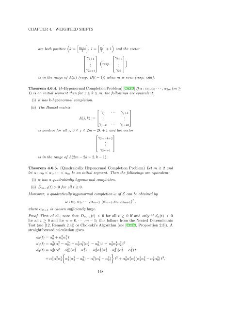
Theorem 4.6.5. (Quadraically Hyponormal Completion Problem) Let m ≥ 2 and
let α : α 0 < α 1 , · · · < α m be an initial segment. Then the followings are equivalent:
(i) α has a quadratically hyponormal completion.
(ii) D m−1 (t) > 0 for all t ≥ 0.
Moreover, a quadratically hyponormal completion ω of L can be obtained by
where α m+1 is chosen sufficiently large.
⎥
⎦
ω : α 0 , α 1 , · · · , α m−2 (α m−1 , α m , α m+1 ) ∧ ,
Proof. First of all, note that D m−1 (t) > 0 for all t ≥ 0 if and only if d n (t) > 0
for all t ≥ 0 and for n = 0, · · · , m − 1; this follows from the Nested Determinants
Test (see [12, Remark 2.4]) or Choleski’s Algorithm (see [CuF2, Proposition 2.3]). A
straightforward calculation gives
d 0 (t) = α 2 0 + α 2 0α 2 1 t
d 1 (t) = α 2 0(α 2 1 − α 2 0) + α 2 0α 2 1(α 2 2 − α 2 0) t + α 2 0α 4 1α 2 2 t 2
d 2 (t) = α0(α 2 1 2 − α0)(α 2 2 2 − α1) 2 + α0α 2 2(α 2 1 2 − α0)(α 2 3 2 − α1) 2 t
{
}
+ α0α 2 1α 2 2
2 α3(α 2 2 2 − α0) 2 − α1(α 2 1 2 − α0)
2 t 2 + α0α 2 1α 4 2(α 2 2α 2 3 2 − α1α 2 0) 2 t 3 ,
148