1998 - Draper Laboratory

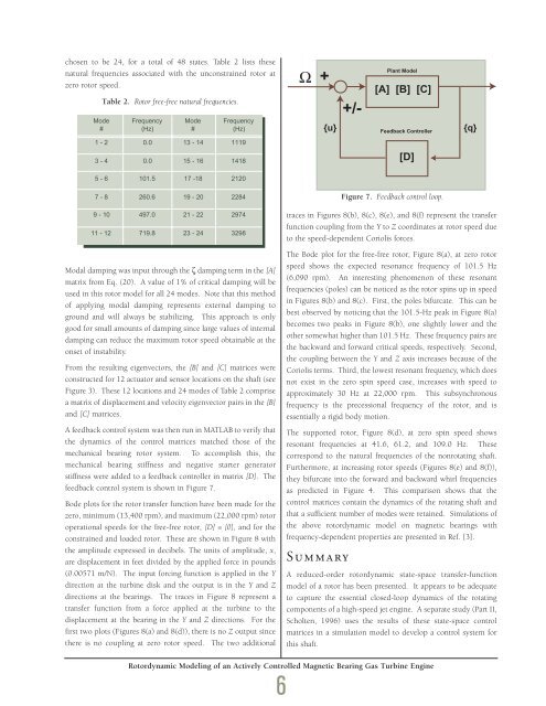
chosen to be 24, for a total of 48 states. Table 2 lists thesenatural frequencies associated with the unconstrained rotor atzero rotor speed.Table 2. Rotor free-free natural frequencies.Ω++/-Plant Model[A] [B] [C]{u}Feedback Controller{q}[D]Figure 7. Feedback control loop.traces in Figures 8(b), 8(c), 8(e), and 8(f) represent the transferfunction coupling from the Y to Z coordinates at rotor speed dueto the speed-dependent Coriolis forces.Modal damping was input through the ζ damping term in the [A]matrix from Eq. (20). A value of 1% of critical damping will beused in this rotor model for all 24 modes. Note that this methodof applying modal damping represents external damping toground and will always be stabilizing. This approach is onlygood for small amounts of damping since large values of internaldamping can reduce the maximum rotor speed obtainable at theonset of instability.From the resulting eigenvectors, the [B] and [C] matrices wereconstructed for 12 actuator and sensor locations on the shaft (seeFigure 3). These 12 locations and 24 modes of Table 2 comprisea matrix of displacement and velocity eigenvector pairs in the [B]and [C] matrices.A feedback control system was then run in MATLAB to verify thatthe dynamics of the control matrices matched those of themechanical bearing rotor system. To accomplish this, themechanical bearing stiffness and negative starter generatorstiffness were added to a feedback controller in matrix [D]. Thefeedback control system is shown in Figure 7.Bode plots for the rotor transfer function have been made for thezero, minimum (13,400 rpm), and maximum (22,000 rpm) rotoroperational speeds for the free-free rotor, [D] = [0], and for theconstrained and loaded rotor. These are shown in Figure 8 withthe amplitude expressed in decibels. The units of amplitude, x,are displacement in feet divided by the applied force in pounds(0.00571 m/N). The input forcing function is applied in the Ydirection at the turbine disk and the output is in the Y and Zdirections at the bearings. The traces in Figure 8 represent atransfer function from a force applied at the turbine to thedisplacement at the bearing in the Y and Z directions. For thefirst two plots (Figures 8(a) and 8(d)), there is no Z output sincethere is no coupling at zero rotor speed. The two additionalThe Bode plot for the free-free rotor, Figure 8(a), at zero rotorspeed shows the expected resonance frequency of 101.5 Hz(6,090 rpm). An interesting phenomenon of these resonantfrequencies (poles) can be noticed as the rotor spins up in speedin Figures 8(b) and 8(c). First, the poles bifurcate. This can bebest observed by noticing that the 101.5-Hz peak in Figure 8(a)becomes two peaks in Figure 8(b), one slightly lower and theother somewhat higher than 101.5 Hz. These frequency pairs arethe backward and forward critical speeds, respectively. Second,the coupling between the Y and Z axis increases because of theCoriolis terms. Third, the lowest resonant frequency, which doesnot exist in the zero spin speed case, increases with speed toapproximately 30 Hz at 22,000 rpm. This subsynchronousfrequency is the precessional frequency of the rotor, and isessentially a rigid body motion.The supported rotor, Figure 8(d), at zero spin speed showsresonant frequencies at 41.6, 61.2, and 109.0 Hz. Thesecorrespond to the natural frequencies of the nonrotating shaft.Furthermore, at increasing rotor speeds (Figures 8(e) and 8(f)),they bifurcate into the forward and backward whirl frequenciesas predicted in Figure 4. This comparison shows that thecontrol matrices contain the dynamics of the rotating shaft andthat a sufficient number of modes were retained. Simulations ofthe above rotordynamic model on magnetic bearings withfrequency-dependent properties are presented in Ref. [3].SummaryA reduced-order rotordynamic state-space transfer-functionmodel of a rotor has been presented. It appears to be adequateto capture the essential closed-loop dynamics of the rotatingcomponents of a high-speed jet engine. A separate study (Part II,Scholten, 1996) uses the results of these state-space controlmatrices in a simulation model to develop a control system forthis shaft.Rotordynamic Modeling of an Actively Controlled Magnetic Bearing Gas Turbine Engine6