1998 - Draper Laboratory

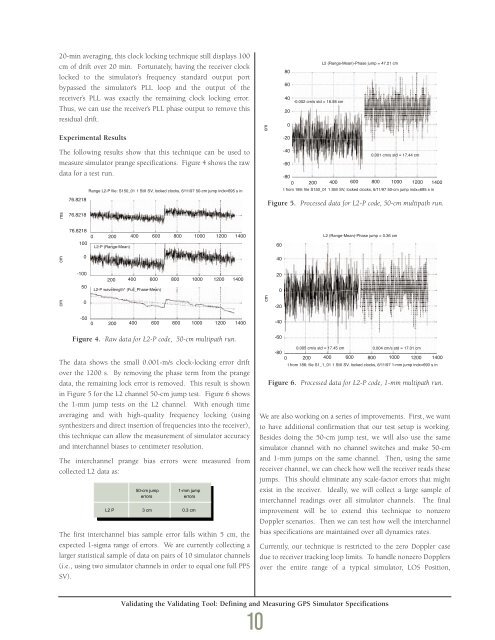
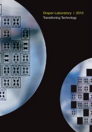
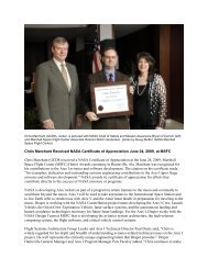
20-min averaging, this clock locking technique still displays 100cm of drift over 20 min. Fortunately, having the receiver clocklocked to the simulator’s frequency standard output portbypassed the simulator’s PLL loop and the output of thereceiver’s PLL was exactly the remaining clock locking error.Thus, we can use the receiver’s PLL phase output to remove thisresidual drift.Experimental ResultsThe following results show that this technique can be used tomeasure simulator prange specifications. Figure 4 shows the rawdata for a test run.Figure 5. Processed data for L2-P code, 50-cm multipath run.Figure 4. Raw data for L2-P code, 50-cm multipath run.The data shows the small 0.001-m/s clock-locking error driftover the 1200 s. By removing the phase term from the prangedata, the remaining lock error is removed. This result is shownin Figure 5 for the L2 channel 50-cm jump test. Figure 6 showsthe 1-mm jump tests on the L2 channel. With enough timeaveraging and with high-quality frequency locking (usingsynthesizers and direct insertion of frequencies into the receiver),this technique can allow the measurement of simulator accuracyand interchannel biases to centimeter resolution.The interchannel prange bias errors were measured fromcollected L2 data as:The first interchannel bias sample error falls within 5 cm, theexpected 1-sigma range of errors. We are currently collecting alarger statistical sample of data on pairs of 10 simulator channels(i.e., using two simulator channels in order to equal one full PPSSV).Figure 6. Processed data for L2-P code, 1-mm multipath run.We are also working on a series of improvements. First, we wantto have additional confirmation that our test setup is working.Besides doing the 50-cm jump test, we will also use the samesimulator channel with no channel switches and make 50-cmand 1-mm jumps on the same channel. Then, using the samereceiver channel, we can check how well the receiver reads thesejumps. This should eliminate any scale-factor errors that mightexist in the receiver. Ideally, we will collect a large sample ofinterchannel readings over all simulator channels. The finalimprovement will be to extend this technique to nonzeroDoppler scenarios. Then we can test how well the interchannelbias specifications are maintained over all dynamics rates.Currently, our technique is restricted to the zero Doppler casedue to receiver tracking loop limits. To handle nonzero Dopplersover the entire range of a typical simulator, LOS Position,Validating the Validating Tool: Defining and Measuring GPS Simulator Specifications10