1998 - Draper Laboratory

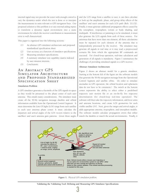
internal signal may not provide the tester with enough control tovary the dynamics under which the test is done or to interpretthe measurements in units relevant to GPS navigation fixes. Ourproposed solution to this problem is to use external aiding inputsto transform a dynamic signal environment into a staticenvironment for which the receiver contribution to measurementerror is well characterized.This paper is organized into the following sections:(1) An abstract GPS simulator architecture and proposedstandardized specification sheet.(2) User accuracy as a function of simulator specifications.(3) Measuring simulator specifications.(4) A summary simulator test capability matrix indexedby user mission interests.(5) Conclusions.An Abstract GPSSimulator Architectureand Proposed StandardizedSpecification SheetSimulation ProblemA GPS simulator generates a facsimile of the GPS signals in spaceas they would be presented to the phase center of each userantenna. This entails many considerations. The simulator mustcreate all the 50-Hz navigation message databits and orbitalinformation available from the Operational Control Segment. Itmust determine the Line Of Sight (LOS) range from each satelliteto each user antenna phase center. It must calculate thedeparture and arrival angles of the LOS vectors relative to thesatellites’ and user’s antenna gain patterns. Given these anglesand the LOS range from a satellite to user, it can then calculateor look up the amplitude, phase, and group delay effects of thesatellites’ and user’s antenna for each LOS path (Refs. [1]-[3]).Finally, it must generate additional propagation effects caused bythe ionosphere, troposphere, terrain or body shading, andmultipath. If interference or jamming is to be simulated, it mustalso generate the LOS signals from each of these sources. Forantennas that have more than one element, all these calculationsmust be repeated for each element of the antenna that isindependently processed by the receiver. The simulator maygenerate all signals in real time or it may read a preprocessedscenario file from which the appropriate RF commands areexecuted. For closed-loop operation, real-time calculation andgeneration of all signals is mandatory. Figure 1 summarizes thechallenges of providing simulated signals to a GPS receiver.Abstract Simulator ArchitectureFigure 2 shows an abstract model for a generic simulator.Starting at the bottom left of the figure are the software modelsthat generate the 50-Hz navigation message from the OperationalControl Segment and satellite orbits. (In order to simulateanomalies in GPS operation, the orbital location and ephemerisdata do not have to be consistent.) The switch at the bottomcenter represents the ability to select either a predefinedtrajectory user motion file or an on-the-fly live trajectorydetermination (for closed-loop real-time operation). Thesoftware will then take the trajectory information, add lever armsand antenna locations, and create LOS geometries for eachvisible satellite (SV). Next, given the ranges and arrival angles, itadds appropriate antenna, troposphere, and ionosphere models.The software models calculate propagation errors that eithermatch the databits or match the actual environments. Finally, itLine of sight: for jth SV,calculate the effects ofSV - user + environment+ antenna (look_angles)on range, carrier, amplitudeTo all SVsionoGround control segment:almanac, ephemeris, databituploads plus actual orbit locationstropoterrainAzi, dep=90-elv lookangles in antennaframe for jth SVUser dynamicspos, vel, acc, jerk,attitude, attituderatesRepeat all neededcalculation for2nd and other antennasNote: Vehicle travels either a known user trajectory orhas an option for on-board Nav system to use GPS + otherdata that can then change the trajectory on-the-flybased on Nav system updates. True closed real-time processingis needed for this case.Figure 1. Physical GPS simulation problem.Validating the Validating Tool: Defining and Measuring GPS Simulator Specifications3