1998 - Draper Laboratory

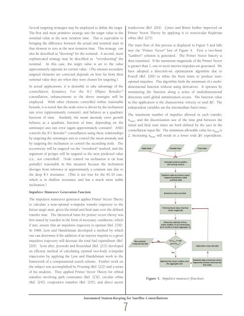
Several targeting strategies may be employed to define the target.The first and most primitive strategy sets the target value to thenominal value at the next iteration time. This is equivalent tobringing the difference between the actual and nominal state inthat element to zero at the next iteration time. This strategy canalso be described as "shooting" for the nominal. A second, moresophisticated strategy may be described as "overshooting" thenominal. In this case, the target value is set to the valueapproximately opposite its current value. (The amount secondarytargeted elements are corrected depends on how far from theirnominal value they are when they were chosen for targeting.)In actual applications, it is desirable to take advantage of theconstellation dynamics. For the 8:1 Ellipso Borealis TMconstellation, enhancements to the above strategies will beemployed. With other elements controlled within reasonablebounds, it is noted that the node error is driven by the inclinationrate error (approximately constant), and behaves as a quadraticfunction of time. Similarly, the mean anomaly error growthbehaves as a quadratic function of time, depending on thesemimajor axis rate error (again approximately constant). ASKScontrols the 8:1 Borealis TM constellation using these relationshipsby targeting the semimajor axis to control the mean anomaly andby targeting the inclination to control the ascending node. Theeccentricity will be targeted via the "overshoot" method, and theargument of perigee will be targeted to the next predicted value(i.e., not controlled). Node control via inclination is (at leastpartially) reasonable in this situation because the inclinationdiverges from reference at approximately a constant rate due tothe deep 8:1 resonance. (This is not true for the 81:10 case,which is in shallow resonance and has a much more stableinclination.)Impulsive Maneuver Generation FunctionThe impulsive maneuver generator applies Primer Vector Theoryto calculate a near-optimal n-impulse transfer trajectory to thefuture target state, given the initial and final state over the definedtransfer time. The theoretical basis for primer vector theory wasfirst stated by Lawden in the form of necessary conditions, whichif met, ensure that an impulsive trajectory is optimal (Ref. [19]).In 1968, Lion and Handelsman developed a method by whichone can determine if the addition of an interior impulse to a givenimpulsive trajectory will decrease the total fuel expenditure (Ref.[20]). Soon after, Jezewski and Rozendaal (Ref. [21]) developedan efficient method of calculating optimal two-body n-impulsetrajectories by applying the Lion and Handelsman work in theframework of a computational search scheme. Further work onthe subject was accomplished by Prussing (Ref. [22]) and a seriesof his students. They applied Primer Vector Theory for orbitaltransfers involving path constraints (Ref. [23]), circular orbits(Ref. [24]), cooperative transfers (Ref. [25]), and direct ascentrendezvous (Ref. [26]). Carter and Brient further improved onPrimer Vector Theory by applying it to noncircular Keplerianorbits (Ref. [27]).The main flow of this process is displayed in Figure 5 and fallsinto the "Primer Vector" box of Figure 4. First a two-burn"Lambert" solution is generated. The Primer Vector history isthen examined. If the maximum magnitude of the Primer Vectoris greater than 1, one or more interior impulses are generated. Wehave adopted a direction-set optimization algorithm due toPowell (Ref. [28]) to refine the burn times to produce nearoptimalimpulses. This algorithm finds the minimum of a multidimensionalfunction without using derivatives. It operates byminimizing the function along a series of multidimensionaldirections until global minimization occurs. The function valuein this application is the characteristic velocity or total ∆V. Theindependent variables are the intermediate burn times.The maximum number of impulses allowed in each transfer,n max , and the discretization size of the time grid between theinitial and final state times are both defined by the user in theconstellation input file. The minimum allowable value for n max is2. Increasing n max will result in a lower total ∆V expenditure.Near-optimaln-impulse burnlistInitial state Transfer time Final stateNoCalculate terminal positionand velocity vectorsEstablish state and primer vectortrajectories between initialand final stateDetermine 2-burn burnlistFind maximum value of primervector magnitudeDetermine estimate of timewhere addition of an intermediateburn results in lowest aggregate ∆VIs |λ| max >1 andand n