- Page 2: TWO-PHASE REACTIVE TRANSPORTOF AN O
- Page 5 and 6: Dit proefschrift is goedgekeurd doo
- Page 7 and 8: 4. The effect of pH on mass transfe
- Page 9 and 10: Samenvatting . . . . . . . . . . .
- Page 11 and 12: 2 1. Introductionproducerbarrierlow
- Page 13 and 14: 4 1. IntroductionTwo inter-European
- Page 16: Part ITwo-phase bulk systems7
- Page 19 and 20: 10 2. Coupled mass transfer and sol
- Page 21 and 22: 12 2. Coupled mass transfer and sol
- Page 23 and 24: 14 2. Coupled mass transfer and sol
- Page 25 and 26: 16 2. Coupled mass transfer and sol
- Page 27 and 28: 18 2. Coupled mass transfer and sol
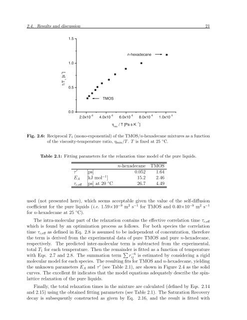
- Page 29: 20 2. Coupled mass transfer and sol
- Page 33 and 34: 24 2. Coupled mass transfer and sol
- Page 35 and 36: 26 2. Coupled mass transfer and sol
- Page 37 and 38: 28 2. Coupled mass transfer and sol
- Page 39 and 40: 30 2. Coupled mass transfer and sol
- Page 41 and 42: 32 3. Interfacial effects during re
- Page 43 and 44: 34 3. Interfacial effects during re
- Page 45 and 46: 36 3. Interfacial effects during re
- Page 47 and 48: 38 3. Interfacial effects during re
- Page 49 and 50: 40 3. Interfacial effects during re
- Page 51 and 52: 42 3. Interfacial effects during re
- Page 53 and 54: 0+,44 4. The effect of pH on mass t
- Page 55 and 56: 46 4. The effect of pH on mass tran
- Page 57 and 58: 48 4. The effect of pH on mass tran
- Page 59 and 60: 50 4. The effect of pH on mass tran
- Page 61 and 62: 52 4. The effect of pH on mass tran
- Page 63 and 64: 54 4. The effect of pH on mass tran
- Page 65 and 66: 56 4. The effect of pH on mass tran
- Page 67 and 68: 58 5. Cross-linking of silica with
- Page 69 and 70: 60 5. Cross-linking of silica with
- Page 71 and 72: 0+,62 5. Cross-linking of silica wi
- Page 73 and 74: 64 5. Cross-linking of silica with
- Page 75 and 76: 66 5. Cross-linking of silica with
- Page 77 and 78: 68 5. Cross-linking of silica with
- Page 79 and 80: 70 5. Cross-linking of silica with
- Page 81 and 82:
72 5. Cross-linking of silica with
- Page 84:
Part IIGel placement in porous mate
- Page 87 and 88:
78 6. Coupled mass transfer and gel
- Page 89 and 90:
80 6. Coupled mass transfer and gel
- Page 91 and 92:
82 6. Coupled mass transfer and gel
- Page 93 and 94:
84 6. Coupled mass transfer and gel
- Page 95 and 96:
86 6. Coupled mass transfer and gel
- Page 97 and 98:
88 6. Coupled mass transfer and gel
- Page 99 and 100:
90 6. Coupled mass transfer and gel
- Page 101 and 102:
92 6. Coupled mass transfer and gel
- Page 103 and 104:
94 6. Coupled mass transfer and gel
- Page 105 and 106:
96 6. Coupled mass transfer and gel
- Page 107 and 108:
98 7. Permeability reduction in por
- Page 109 and 110:
100 7. Permeability reduction in po
- Page 111 and 112:
102 7. Permeability reduction in po
- Page 113 and 114:
104 7. Permeability reduction in po
- Page 115 and 116:
106 7. Permeability reduction in po
- Page 117 and 118:
108 7. Permeability reduction in po
- Page 119 and 120:
110 7. Permeability reduction in po
- Page 121 and 122:
112 7. Permeability reduction in po
- Page 123 and 124:
114 8. Model of reactive transport
- Page 125 and 126:
116 8. Model of reactive transport
- Page 127 and 128:
118 8. Model of reactive transport
- Page 129 and 130:
120 8. Model of reactive transport
- Page 131 and 132:
122 8. Model of reactive transport
- Page 133 and 134:
124 8. Model of reactive transport
- Page 135 and 136:
126 8. Model of reactive transport
- Page 137 and 138:
128 8. Model of reactive transport
- Page 139 and 140:
130 8. Model of reactive transport
- Page 141 and 142:
132 9. Concluding remarks and outlo
- Page 143 and 144:
134 9. Concluding remarks and outlo
- Page 145 and 146:
136 9. Concluding remarks and outlo
- Page 147 and 148:
138 9. Concluding remarks and outlo
- Page 149 and 150:
140
- Page 151 and 152:
-142 Appendix A, - C D *, - D
- Page 153 and 154:
144 Appendix Awhere S 0 is a consta
- Page 155 and 156:
146 Appendix AThe 0.95 Tesla scanne
- Page 157 and 158:
148 Appendix B
- Page 159 and 160:
150 Appendix CwhereΩ A (θ) = −2
- Page 161 and 162:
152 Appendix C
- Page 163 and 164:
154 Appendix D
- Page 165 and 166:
156 Appendix Eand equal to zero in
- Page 167 and 168:
158 Appendix EAs the saturations, d
- Page 169 and 170:
160 Bibliography[12] B. Vinot, R. S
- Page 171 and 172:
162 Bibliography[40] M. D. Mantle a
- Page 173 and 174:
164 Bibliography[70] F. J. M. van d
- Page 175 and 176:
166 Bibliography[97] K. Yoshida, A.
- Page 177 and 178:
168 Bibliography[127] G. W. Scherer
- Page 179 and 180:
170 Bibliography
- Page 181 and 182:
172 Summaryand gelation rates. The
- Page 183 and 184:
174 Samenvattingwaterfase. De T 1 v
- Page 185 and 186:
176 List of publications
- Page 187 and 188:
178 Dankwoordimmer opgewekte stemmi
- Page 189:
Prior to the speech, Harald Cramér