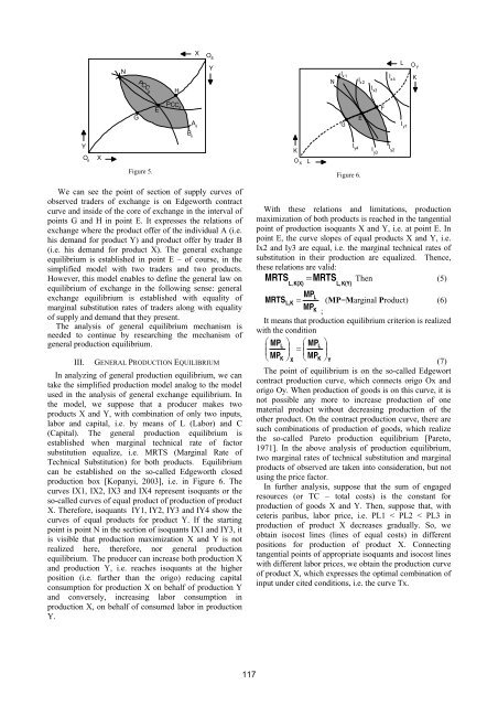
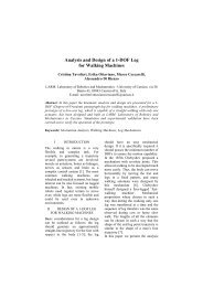
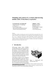
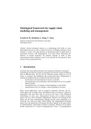
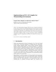
In the two-dimensional model of consumers’ choice limitsor the so-called budget consumption limitation areexpressed by the so-called line or consumption limit. Incase that the variables of money income of traders A andB are equal in exchange, i.e. IA = IB, and prices ofproperties X and Y which come in exchange betweenthem Px and Py, the budget limitation of consumption forboth exchangers can be expressed by the relation:IA, B= X⋅P+ Y⋅P X Ywhence(1)X =Y =IPXIPYP−PXXP−PXY⋅ Y⋅ XUnder the above supposition, the identical budget linecan present the limits of consumers’ choice for traders Aand B. With unchanged prices of goods and amount ofmoney income, the position of budget line remainsunchanged, and its slope expresses the relation of propertyprices, i.e. Px and Py. Look now at Figure 3, thepossibilities of general equilibrium in exchange, takinginto consideration the amount of money income and pricesof exchanged goodsFigure 3.In Figure 3, general exchange equilibrium between Aand B is at point E on the Egdeworth contract curve. Atthis point, namely, we have matching up the slopes ofindifference curves of trader A, on the curve Ae and theslope of indifference curve B, the other trader inexchange. In this point (as in all other points of thecontract curve), we have matching up of marginalsubstitution rates of X and Y for traders A and B.However, contrary to other points on the contract curve, inE, the slope of their marginal substitution slope, i. e. MRS(it is in fact the slope of tangent in some point) ismatching up with the slope of their budget line. The slopeof budget line expresses relative prices, in other words, therelation of prices of goods in exchange, i.e. X and Y. Atthe equilibrium point E, the following equalities are valid:PXMUXMRS A(X,Y) = MRSB(X,Y)= =PYMUY(4)(MU – Marginal Utility)At point E, equilibrium goods prices have the samemutual relations in marginal rate of goods substitution, i.e.MRS is equal for both traders in exchange, and at the(2)(3)same time, it is appropriate to relations of marginal utilityof exchanged goods. It means that the equilibrium point Eis suitable for relation of the proportion where supply anddemand of exchanged goods become equal.YI/P xA 1I/P y A 2 A3 BE 1b2I/P y1E b3B 2E a3PCC AI/P y2B 3O AEa1E a2XE b1I/P x1I/P x2I/P x3 XFigure 4.By the combination of indifference curves and budgetlines we obtain the so-called PCC (Price ConsumptionCurve), which show the structure of optimal consumerbaskets in case of price changes of some goods (supposingthat prices of other goods, the level of money incomes ofconsumers and their preference system are steady). InFigure 4, we presented the curves of relations of pricesand consumption for individuals A and B, supposing thatthe product price X changes for trader A; for trader B, theproduct price Y is changeable. All other relations andconditions remain unchangeable.The curve of relations of price and consumption oftrader A, i.e. curve PCCA shows that, starting from thecombination of goods in point Ea1, which is located alongwith the starting position of budget line, the trader A isready to offer increasing quantity of product X forincreasing less quantity of product Y. It is done bygradually price reduction of product X presented bybudget lines I/Px2 and I/Px3. This trader tries to optimizehis consumer utility in the conditions of changed prices.Contrary to trader A, in northeast angle of Diagram,considering PCCB, i.e. the curve of relations of price andconsumptions of trader B, we see that the latter trader isready to exchange more product Y whose price reducesfor increasingly less quantity of product X, in view ofmaximization of his consumer utility.In fact, the curve of relations of prices and consumption ofthe trader A, i. e. PCCA, represents the curve of offer A,i.e. its readiness to change goods X for Y in exchange. Onthe other side PCCB, i.e. the curve of relations of pricesand consumption of trader B, presents the curve of offerB, i.e. acceptable relation of goods exchange X and Y forIndividual B, depending on price change of product Y.Traders of exchange A and B along their offer curves,starting from points Ea1 and Eb1 to points Ea3 and Eb3get to indifference curves which become more distantfrom the origos, i.e. which express an increasing level ofutility for them.Present, finally, in Figure 5, the curve of relations ofprices and consumption of both traders, i.e. PCCA andPCCB, inside of the so-called “region of mutualadvantages”, limited by their starting indifference curvesAe and Be.PCC BYO BI/P y3116
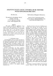
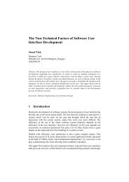
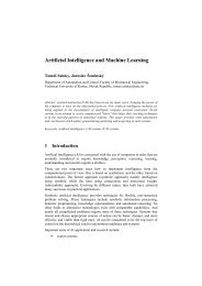
NPCC BHXOBYNI x1I x2I x3I x4LO YKYO AXGFigure 5.EPCC AB eA eKO XLFEGI y1I y4 Iy3I y2Figure 6.We can see the point of section of supply curves ofobserved traders of exchange is on Edgeworth contractcurve and inside of the core of exchange in the interval ofpoints G and H in point E. It expresses the relations ofexchange where the product offer of the individual A (i.e.his demand for product Y) and product offer by trader B(i.e. his demand for product X). The general exchangeequilibrium is established in point E – of course, in thesimplified model with two traders and two products.However, this model enables to define the general law onequilibrium of exchange in the following sense: generalexchange equilibrium is established with equality ofmarginal substitution rates of traders along with equalityof supply and demand that they present.The analysis of general equilibrium mechanism isneeded to continue by researching the mechanism ofgeneral production equilibrium.III. GENERAL PRODUCTION EQUILIBRIUMIn analyzing of general production equilibrium, we cantake the simplified production model analog to the modelused in the analysis of general exchange equilibrium. Inthe model, we suppose that a producer makes twoproducts X and Y, with combination of only two inputs,labor and capital, i.e. by means of L (Labor) and C(Capital). The general production equilibrium isestablished when marginal technical rate of factorsubstitution equalize, i.e. MRTS (Marginal Rate ofTechnical Substitution) for both products. Equilibriumcan be established on the so-called Edgeworth closedproduction box [Kopanyi, 2003], i.e. in Figure 6. Thecurves IX1, IX2, IX3 and IX4 represent isoquants or theso-called curves of equal product of production of productX. Therefore, isoquants IY1, IY2, IY3 and IY4 show thecurves of equal products for product Y. If the startingpoint is point N in the section of isoquants IX1 and IY3, itis visible that production maximization X and Y is notrealized here, therefore, nor general productionequilibrium. The producer can increase both production Xand production Y, i.e. reaches isoquants at the higherposition (i.e. further than the origo) reducing capitalconsumption for production X on behalf of production Yand conversely, increasing labor consumption inproduction X, on behalf of consumed labor in productionY.With these relations and limitations, productionmaximization of both products is reached in the tangentialpoint of production isoquants X and Y, i.e. at point E. Inpoint E, the curve slopes of equal products X and Y, i.e.Ix2 and Iy3 are equal, i.e. the marginal technical rates ofsubstitution in their production are equalized. Thence,these relations are valid:MRTS = MRTS Then (5)L, K(X)MPMRTS L,K =MPLKL, K(Y)(MP=Marginal Product) (6);It means that production equilibrium criterion is realizedwith the condition⎛ MPL⎞⎜MP⎟⎝ K ⎠⎛ MPL⎞=⎜MP⎟⎝ K ⎠XY(7)The point of equilibrium is on the so-called Edgewortcontract production curve, which connects origo Ox andorigo Oy. When production of goods is on this curve, it isnot possible any more to increase production of onematerial product without decreasing production of theother product. On the contract production curve, there aresuch combinations of production of goods, which realizethe so-called Pareto production equilibrium [Pareto,1971]. In the above analysis of production equilibrium,two marginal rates of technical substitution and marginalproducts of observed are taken into consideration, but notusing the price factor.In further analysis, suppose that the sum of engagedresources (or TC – total costs) is the constant forproduction of goods X and Y. Then, suppose that, withceteris paribus, labor price, i.e. PL1 < PL2 < PL3 inproduction of product X decreases gradually. So, weobtain isocost lines (lines of equal costs) in differentpositions for production of product X. Connectingtangential points of appropriate isoquants and isocost lineswith different labor prices, we obtain the production curveof product X, which expresses the optimal combination ofinput under cited conditions, i.e. the curve Tx.117
- Page 1 and 2:
4 4 th IEEE International Symposium
- Page 3 and 4:
EXPRES 20124 th International Sympo
- Page 5 and 6:
Application of Thermopile Technolog
- Page 7 and 8:
Design of a Solar Hybrid System....
- Page 9 and 10:
___________________________________
- Page 11 and 12:
environmental protection and global
- Page 13 and 14:
But can we use the human body sweat
- Page 15 and 16:
IX. REFERENCES[1] Todorovic B. Cvje
- Page 17 and 18:
QQ⎛ Λt⎞=⎜⎟⎝ Λ ⎠Nt Nwh
- Page 19 and 20:
Analysis of the Energy-Optimum of H
- Page 21 and 22:
V. OBJECTIVE FUNCTIONThe objective
- Page 23 and 24:
The Set-Up Geometry of Sun Collecto
- Page 25 and 26:
continuous east-west sun collector
- Page 27 and 28:
continuously measure the thermal ch
- Page 29 and 30:
CEvaluation of measurement resultsA
- Page 31 and 32:
Application of Thermopile Technolog
- Page 33 and 34:
Temperature of the components [C]90
- Page 35 and 36:
nighttime, to weather or to the cha
- Page 37 and 38:
η uη u0.50.40.30.20.1T 1 - 400K0.
- Page 39 and 40:
Figure 10. . SPS Concept illustrati
- Page 41 and 42:
[16] Zoya B. Popović: Wireless Pow
- Page 43 and 44:
25.0020.0015.0010.005.000.00Figure
- Page 45 and 46:
· ℃ 0.0738 · 1.209 0.0892
- Page 47 and 48:
use may be advantageous not only in
- Page 49 and 50:
To find the reasons for this disagr
- Page 51 and 52:
Toward Future: Positive Net-Energy
- Page 53 and 54:
EnergyPlus environment, we used mod
- Page 55 and 56:
To keep future energy consumption d
- Page 57 and 58:
A New Calculation Method to Analyse
- Page 59 and 60:
On Fig. 3. can be seen the areas th
- Page 61 and 62:
Present and Future of Geothermal En
- Page 63 and 64:
TABLE II.THE TEMPERATURE DATA AND C
- Page 65 and 66:
Error in Water Meter Measuring at W
- Page 67 and 68: III.RESULTS OF MEASURMENTSEach meas
- Page 69 and 70: TABLE I.THE AVERAGE VALUE OF THERMA
- Page 71 and 72: If the walls of the DHEs are made o
- Page 73 and 74: Environmental External Costs Associ
- Page 75 and 76: iodiesel production facility with a
- Page 77 and 78: Contribution of unit processesto ex
- Page 79 and 80: Heat Pump News in HungaryBéla Ád
- Page 81 and 82: Thermal Comfort Measurements In Lar
- Page 83 and 84: IV.DISCUSSIONThe sample frequencies
- Page 85 and 86: For a Clear View of Traditional and
- Page 87 and 88: esults in geographically distribute
- Page 89 and 90: Design of a Solar Hybrid SystemMari
- Page 91 and 92: Maintaining the set point temperatu
- Page 93 and 94: Decision system theory model of ope
- Page 95 and 96: parameter of pump in the function o
- Page 97 and 98: Importance and Value of Predictive
- Page 99 and 100: D. Overview of existing boiler oper
- Page 101 and 102: HEAVY FUEL OIL FIRED, STEAMNATURAL
- Page 103 and 104: MATHEMATICAL MODEL AND NUMERICAL SI
- Page 105 and 106: C. Energy balance equationMathemati
- Page 107 and 108: Discretization energy balance equat
- Page 109 and 110: T ulf=32 º C, A - m =0.00162 kg/s,
- Page 111 and 112: Comparison of Heat Pump and MicroCH
- Page 113 and 114: the microCHP development. The energ
- Page 115 and 116: control and stabilizer must be deve
- Page 117: In Figure 1, in relation to the ord
- Page 121 and 122: exchange, as in reality, economies
- Page 123 and 124: esponsibilities for consequences, o
- Page 125 and 126: Coca-Cola Enterprise Inc had approx
- Page 127 and 128: Flow Pattern Map for In Tube Evapor
- Page 129 and 130: circumference with a liquid film. T
- Page 131 and 132: Tube diameter: d 6 mm W Heat flux
- Page 133 and 134: Realization of Concurrent Programmi
- Page 135 and 136: applications the development, optim
- Page 137 and 138: Renewable energy sources in automob
- Page 139 and 140: commercial arrays can be built at b
- Page 141 and 142: of multiple thin films produced usi
- Page 143: EXPRES 20124 th International Sympo