ASReml-S reference manual - VSN International

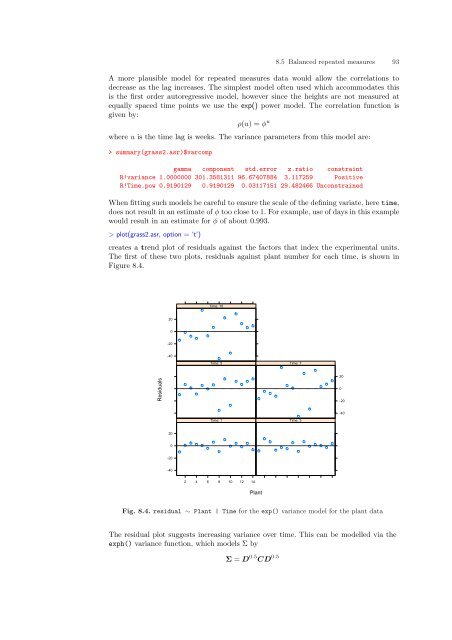
8.5 Balanced repeated measures 93A more plausible model for repeated measures data would allow the correlations todecrease as the lag increases. The simplest model often used which accommodates thisis the first order autoregressive model, however since the heights are not measured atequally spaced time points we use the exp() power model. The correlation function isgiven by:ρ(u) = φ uwhere u is the time lag is weeks. The variance parameters from this model are:> summary(grass2.asr)$varcompgamma component std.error z.ratio constraintR!variance 1.0000000 301.3581311 96.67407884 3.117259 PositiveR!Time.pow 0.9190129 0.9190129 0.03117151 29.482466 UnconstrainedWhen fitting such models be careful to ensure the scale of the defining variate, here time,does not result in an estimate of φ too close to 1. For example, use of days in this examplewould result in an estimate for φ of about 0.993.> plot(grass2.asr, option = ’t’)creates a trend plot of residuals against the factors that index the experimental units.The first of these two plots, residuals against plant number for each time, is shown inFigure 8.4.Time: 10200-20-40Time: 5Time: 7Residuals200-20-40Time: 1 Time: 3200-20-402 4 6 8 10 12 14PlantFig. 8.4. residual ∼ Plant | Time for the exp() variance model for the plant dataThe residual plot suggests increasing variance over time. This can be modelled via theexph() variance function, which models Σ byΣ = D 0.5 CD 0.5