ASReml-S reference manual - VSN International

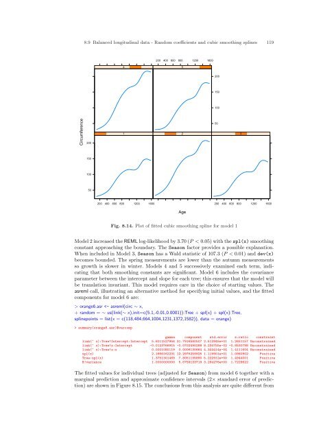
8.9 Balanced longitudinal data - Random coefficients and cubic smoothing splines 119200 400 600 800 1200 160045200150100Circumference2001 250315010050200 400 600 800 1200 1600200 400 600 800 1200 1600AgeFig. 8.14. Plot of fitted cubic smoothing spline for model 1Model 2 increased the REML log-likelihood by 3.70 (P < 0.05) with the spl(x) smoothingconstant approaching the boundary. The Season factor provides a possible explanation.When included in Model 3, Season has a Wald statistic of 107.3 (P < 0.01) and dev(x)becomes bounded. The spring measurements are lower than the autumn measurementsso growth is slower in winter. Models 4 and 5 successively examined each term, indicatingthat both smoothing constants are significant. Model 6 includes the covarianceparameter between the intercept and slope for each tree; this ensures that the model willbe translation invariant. This model requires care in the choice of starting values. Theasreml call, illustrating an alternative method for specifying initial values, and the fittedcomponents for model 6 are:> orange6.asr summary(orange6.asr)$varcompgamma component std.error z.ratio constraintlink(~ x):Tree!Intercept:Intercept 5.6011527956 31.7916580507 2.512945e+01 1.2651157 Unconstrainedlink(~ x):Tree!x:Intercept -0.0123766915 -0.0702490288 8.234755e-02 -0.8530798 Unconstrainedlink(~ x):Tree!x:x 0.0001080119 0.0006130664 4.344414e-04 1.4111604 Unconstrainedspl(x) 2.1666162231 12.2975259925 1.119901e+01 1.0980902 PositiveTree:spl(x) 1.3751301469 7.8051195890 5.222912e+00 1.4944001 PositiveR!variance 1.0000000000 5.6759133719 3.294276e+00 1.7229622 PositiveThe fitted values for individual trees (adjusted for Season) from model 6 together with amarginal prediction and approximate confidence intervals (2× standard error of prediction)are shown in Figure 8.15. The conclusions from this analysis are quite different from