ASReml-S reference manual - VSN International

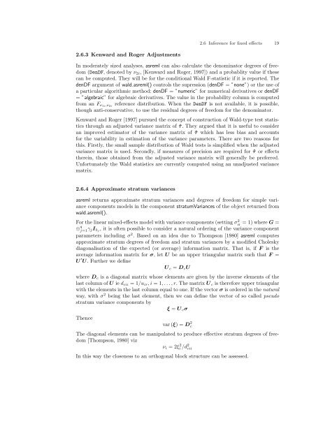
2.6 Inference for fixed effects 192.6.3 Kenward and Roger AdjustmentsIn moderately sized analyses, asreml can also calculate the denominator degrees of freedom(DenDF, denoted by ν 2i , [Kenward and Roger, 1997]) and a probablity value if thesecan be computed. They will be for the conditional Wald F-statistic if it is reported. ThedenDF argument of wald.asreml() controls the supression (denDF = ”none”) or the use ofa particular algorithmic method: denDF = ”numeric” for numerical derivatives or denDF= ”algebraic” for algebraic derivatives. The value in the probability column is computedfrom an F ν1i ,ν 2ireference distribution. When the DenDF is not available, it is possible,though anti-conservative, to use the residual degrees of freedom for the denominator.Kenward and Roger [1997] pursued the concept of construction of Wald-type test statisticsthrough an adjusted variance matrix of ˆτ . They argued that it is useful to consideran improved estimator of the variance matrix of ˆτ which has less bias and accountsfor the variability in estimation of the variance parameters. There are two reasons forthis. Firstly, the small sample distribution of Wald tests is simplified when the adjustedvariance matrix is used. Secondly, if measures of precision are required for ˆτ or effectstherein, those obtained from the adjusted variance matrix will generally be preferred.Unfortunately the Wald statistics are currently computed using an unadjusted variancematrix.2.6.4 Approximate stratum variancesasreml returns approximate stratum variances and degrees of freedom for simple variancecomponents models in the component stratumVariances of the object returned fromwald.asreml().For the linear mixed-effects model with variance components (setting σ 2 = 1) where G =H⊕ q j=1 γ jI bj , it is often possible to consider a natural ordering of the variance componentparameters including σ 2 . Based on an idea due to Thompson [1980] asreml computesapproximate stratum degrees of freedom and stratum variances by a modified Choleskydiagonalisation of the expected (or average) information matrix. That is, if F is theaverage information matrix for σ, let U be an upper triangular matrix such that F =U ′ U. Further we defineU c = D c Uwhere D c is a diagonal matrix whose elements are given by the inverse elements of thelast column of U ie d cii = 1/u ir , i = 1, . . . , r. The matrix U c is therefore upper triangularwith the elements in the last column equal to one. If the vector σ is ordered in the naturalway, with σ 2 being the last element, then we can define the vector of so called pseudostratum variance components byξ = U c σThencevar (ξ) = D 2 cThe diagonal elements can be manipulated to produce effective stratum degrees of freedom[Thompson, 1980] vizν i = 2ξ 2 i /d 2 ciiIn this way the closeness to an orthogonal block structure can be assessed.