ASReml-S reference manual - VSN International

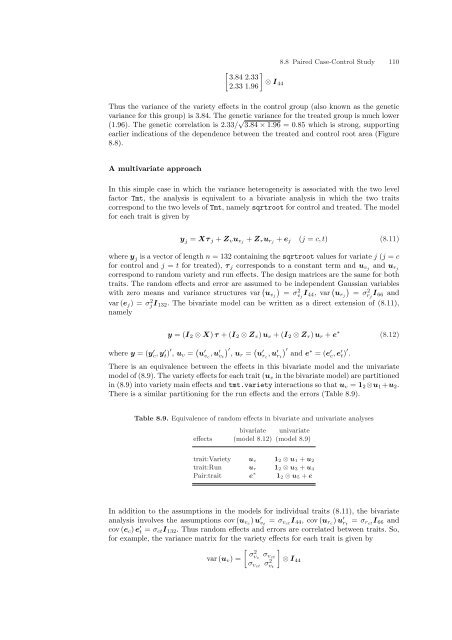
8.8 Paired Case-Control Study 110[ ]3.84 2.33⊗ I2.33 1.96 44Thus the variance of the variety effects in the control group (also known as the geneticvariance for this group) is 3.84. The genetic variance for the treated group is much lower(1.96). The genetic correlation is 2.33/ √ 3.84 × 1.96 = 0.85 which is strong, supportingearlier indications of the dependence between the treated and control root area (Figure8.8).A multivariate approachIn this simple case in which the variance heterogeneity is associated with the two levelfactor Tmt, the analysis is equivalent to a bivariate analysis in which the two traitscorrespond to the two levels of Tmt, namely sqrtroot for control and treated. The modelfor each trait is given byy j = Xτ j + Z v u vj + Z r u rj + e j (j = c, t) (8.11)where y j is a vector of length n = 132 containing the sqrtroot values for variate j (j = cfor control and j = t for treated), τ j corresponds to a constant term and u vj and u rjcorrespond to random variety and run effects. The design matrices are the same for bothtraits. The random effects and error are assumed to be independent Gaussian variableswith zero means and variance structures var ( )u vj = σ2vjI 44 , var ( )u rj = σ2rjI 66 andvar (e j ) = σj 2I 132. The bivariate model can be written as a direct extension of (8.11),namelyy = (I 2 ⊗ X) τ + (I 2 ⊗ Z v ) u v + (I 2 ⊗ Z r ) u r + e ∗ (8.12)where y = (y ′ c, y ′ t) ′ , u v = ( u ′ v c, u ′ v t) ′,ur = ( u ′ r c, u ′ r t) ′and e ∗ = (e ′ c, e ′ t) ′ .There is an equivalence between the effects in this bivariate model and the univariatemodel of (8.9). The variety effects for each trait (u v in the bivariate model) are partitionedin (8.9) into variety main effects and tmt.variety interactions so that u v = 1 2 ⊗u 1 +u 2 .There is a similar partitioning for the run effects and the errors (Table 8.9).Table 8.9. Equivalence of random effects in bivariate and univariate analysesbivariate univariateeffects (model 8.12) (model 8.9)trait:Variety u v 1 2 ⊗ u 1 + u 2trait:Run u r 1 2 ⊗ u 3 + u 4Pair:trait e ∗ 1 2 ⊗ u 5 + eIn addition to the assumptions in the models for individual traits (8.11), the bivariateanalysis involves the assumptions cov (u vc ) u ′ v t= σ vct I 44 , cov (u rc ) u ′ r t= σ rct I 66 andcov (e c ) e ′ t = σ ct I 132 . Thus random effects and errors are correlated between traits. So,for example, the variance matrix for the variety effects for each trait is given by[ ]σ2var (u v ) = vcσ vctσ vct σv 2 ⊗ I 44t