- Page 1 and 2:
Rolling bearings
- Page 3 and 4:
Rolling bearings
- Page 5 and 6:
E Bearing specifics ...............
- Page 7 and 8:
7.5 Matched bearings arranged back-
- Page 9 and 10:
7
- Page 11 and 12:
Foreword This catalogue contains th
- Page 13 and 14:
without flange rings er bearings be
- Page 15 and 16:
Units of measurement This catalogue
- Page 17 and 18:
Meeting the toughest challenges Our
- Page 19 and 20:
Bearings SKF is the world leader in
- Page 21:
Bearing basics ....................
- Page 24 and 25:
Bearing basics Selecting rolling be
- Page 26 and 27:
Bearing basics Bearing systems (†
- Page 28 and 29:
Bearing basics Bearing types and de
- Page 30 and 31:
Bearing basics Angular contact ball
- Page 32 and 33: Bearing basics Cylindrical roller b
- Page 34 and 35: Bearing basics Needle roller bearin
- Page 36 and 37: Bearing basics Angular contact thru
- Page 38 and 39: Bearing basics Support rollers (con
- Page 40 and 41: Bearing basics Fig. 7 a b c c d Mac
- Page 42 and 43: Bearing basics Boundary dimensions
- Page 44 and 45: Bearing basics Basic bearing design
- Page 46 and 47: Bearing basics Diagram 3 Designatio
- Page 48 and 49: Bearing basics Basic selection crit
- Page 50 and 51: Bearing basics Loads Fig. 19 Magnit
- Page 52 and 53: Bearing basics Combined loads A com
- Page 54 and 55: Bearing basics Misalignment Angular
- Page 56 and 57: Bearing basics Friction Rolling bea
- Page 58 and 59: Bearing basics Mounting and dismoun
- Page 60 and 61: Bearing basics Sealing solutions To
- Page 63 and 64: Selecting bearing size B A systems
- Page 65 and 66: Bearing life and load ratings Beari
- Page 67 and 68: Selecting bearing size using the li
- Page 69 and 70: 2 Selecting bearing size using the
- Page 71 and 72: Selecting bearing size using the li
- Page 73 and 74: Selecting bearing size using the li
- Page 75 and 76: Selecting bearing size using the li
- Page 77 and 78: Selecting bearing size using the li
- Page 79 and 80: Selecting bearing size using the li
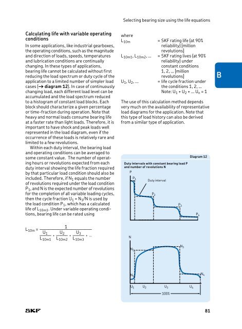
- Page 81: Selecting bearing size using the li
- Page 85 and 86: Selecting bearing size using the li
- Page 87 and 88: Dynamic bearing loads Equivalent dy
- Page 89 and 90: Selecting bearing size using static
- Page 91 and 92: Selecting bearing size using static
- Page 93 and 94: Calculation examples • A more cos
- Page 95 and 96: SKF calculation tools SKF Bearing B
- Page 97: SKF life testing SKF life testing S
- Page 100 and 101: Friction The friction in a rolling
- Page 102 and 103: Friction The SKF model for calculat
- Page 104 and 105: Friction Kinematic replenishment/st
- Page 106 and 107: Friction Table 2a Geometric and loa
- Page 108 and 109: Friction Table 3a Geometric constan
- Page 110 and 111: Friction Table 3e Geometric constan
- Page 112 and 113: Friction Drag losses Bearings lubri
- Page 114 and 115: Friction Drag losses for vertical s
- Page 116 and 117: Friction Starting torque The starti
- Page 119 and 120: Speeds Basics of bearing speed ....
- Page 121 and 122: Reference speed Diagram 1 Heat flow
- Page 123 and 124: Reference speed Diagram 2 Adjustmen
- Page 125 and 126: Reference speed Diagram 4 Adjustmen
- Page 127 and 128: Reference speed Example 1 An SKF Ex
- Page 129 and 130: Special cases Special cases In cert
- Page 131: Vibration generation at high speeds
- Page 134 and 135:
Bearing specifics Dimensions For in
- Page 136 and 137:
Bearing specifics Table 1 Tolerance
- Page 138 and 139:
Bearing specifics Table 2 Diameter
- Page 140 and 141:
Bearing specifics Table 4 P6 class
- Page 142 and 143:
Bearing specifics Table 6 Normal an
- Page 144 and 145:
Bearing specifics Table 8 P5 class
- Page 146 and 147:
Bearing specifics Table 10 Toleranc
- Page 148 and 149:
Bearing specifics Table 12 Normal t
- Page 150 and 151:
Bearing specifics Table 15 Chamfer
- Page 152 and 153:
Bearing specifics The initial inter
- Page 154 and 155:
Bearing specifics Ceramics The comm
- Page 156 and 157:
Bearing specifics Therefore, whethe
- Page 158 and 159:
Bearing specifics Hydrogenated acry
- Page 161 and 162:
Design considerations Bearing syste
- Page 163 and 164:
Bearing systems locating bearing po
- Page 165 and 166:
Bearing systems Adjusted bearing sy
- Page 167 and 168:
Radial location of bearings Radial
- Page 169 and 170:
Radial location of bearings 3. Bear
- Page 171 and 172:
Radial location of bearings Bearing
- Page 173 and 174:
Radial location of bearings Shaft a
- Page 175 and 176:
Radial location of bearings Table 2
- Page 177 and 178:
Radial location of bearings Table 5
- Page 179 and 180:
Radial location of bearings Relatio
- Page 181 and 182:
Radial location of bearings Table 7
- Page 183 and 184:
Radial location of bearings Table 7
- Page 185 and 186:
Radial location of bearings Table 7
- Page 187 and 188:
Radial location of bearings Table 7
- Page 189 and 190:
Radial location of bearings Table 7
- Page 191 and 192:
Radial location of bearings Table 7
- Page 193 and 194:
Radial location of bearings Table 8
- Page 195 and 196:
Radial location of bearings Table 8
- Page 197 and 198:
Radial location of bearings Table 8
- Page 199 and 200:
Radial location of bearings Table 8
- Page 201 and 202:
Radial location of bearings Table 8
- Page 203 and 204:
Radial location of bearings Table 9
- Page 205 and 206:
Radial location of bearings The per
- Page 207 and 208:
Axial location of bearings Locating
- Page 209 and 210:
Axial location of bearings Bearings
- Page 211 and 212:
Axial location of bearings CARB tor
- Page 213 and 214:
Designing associated components Fig
- Page 215 and 216:
Selecting internal clearance or pre
- Page 217 and 218:
Selecting internal clearance or pre
- Page 219 and 220:
Selecting internal clearance or pre
- Page 221 and 222:
Selecting internal clearance or pre
- Page 223 and 224:
Selecting internal clearance or pre
- Page 225 and 226:
Selecting internal clearance or pre
- Page 227 and 228:
Selecting internal clearance or pre
- Page 229 and 230:
Sealing solutions Fig. 43 Fig. 44 S
- Page 231 and 232:
Sealing solutions Integral bearing
- Page 233 and 234:
Sealing solutions External seals Fo
- Page 235 and 236:
Sealing solutions Fig. 57 Fig. 58 F
- Page 237 and 238:
Sealing solutions V-ring seals V-ri
- Page 239:
Sealing solutions F 237
- Page 242 and 243:
Lubrication Basics of lubrication R
- Page 244 and 245:
Lubrication Grease lubrication The
- Page 246 and 247:
Lubrication Lubricating greases Lub
- Page 248 and 249:
Lubrication Temperature zones Tempe
- Page 250 and 251:
Lubrication Protection against corr
- Page 252 and 253:
Lubrication SKF greases - technical
- Page 254 and 255:
Lubrication Relubrication Rolling b
- Page 256 and 257:
Lubrication Very slow speeds Select
- Page 258 and 259:
Lubrication Diagram 4 Relubrication
- Page 260 and 261:
Lubrication Relubrication procedure
- Page 262 and 263:
Lubrication To effectively replace
- Page 264 and 265:
Lubrication Oil lubrication Fig. 6
- Page 266 and 267:
Lubrication Oil jet For very high-s
- Page 268 and 269:
Lubrication Selecting lubricating o
- Page 270 and 271:
20 000 Lubrication Diagram 5 Estima
- Page 273 and 274:
Mounting, dismounting and bearing c
- Page 275 and 276:
General Fig. 1 a b 1 2 a b 1 2 3 4
- Page 277 and 278:
Mounting Mounting Depending on the
- Page 279 and 280:
Mounting Bearing adjustment The int
- Page 281 and 282:
Mounting Fig. 14 the bearing († f
- Page 283 and 284:
Mounting Fig. 18 a c b b a c a Fig.
- Page 285 and 286:
TMEM 1500 Mounting Fig. 22 0.450 ON
- Page 287 and 288:
Dismounting Fig. 23 Dismounting If
- Page 289 and 290:
Dismounting Dismounting bearings fi
- Page 291 and 292:
Dismounting Fig. 32 Fig. 33 H 289
- Page 293 and 294:
Inspection and cleaning Bearing sto
- Page 295:
Deep groove ball bearings 1 Y-beari
- Page 298 and 299:
1 Deep groove ball bearings Designs
- Page 300 and 301:
1 Deep groove ball bearings Double
- Page 302 and 303:
1 Deep groove ball bearings Sealing
- Page 304 and 305:
1 Deep groove ball bearings Low-fri
- Page 306 and 307:
1 Deep groove ball bearings ICOS oi
- Page 308 and 309:
1 Deep groove ball bearings Grease
- Page 310 and 311:
1 Deep groove ball bearings Bearing
- Page 312 and 313:
1 Deep groove ball bearings Perform
- Page 314 and 315:
1 Deep groove ball bearings Bearing
- Page 316 and 317:
1 Deep groove ball bearings Table 6
- Page 318 and 319:
1 Deep groove ball bearings Loads S
- Page 320 and 321:
1 Deep groove ball bearings Tempera
- Page 322 and 323:
1 Deep groove ball bearings Designa
- Page 324 and 325:
1.1 Single row deep groove ball bea
- Page 326 and 327:
1.1 Single row deep groove ball bea
- Page 328 and 329:
1.1 Single row deep groove ball bea
- Page 330 and 331:
1.1 Single row deep groove ball bea
- Page 332 and 333:
1.1 Single row deep groove ball bea
- Page 334 and 335:
1.1 Single row deep groove ball bea
- Page 336 and 337:
1.1 Single row deep groove ball bea
- Page 338 and 339:
1.1 Single row deep groove ball bea
- Page 340 and 341:
1.1 Single row deep groove ball bea
- Page 342 and 343:
1.1 Single row deep groove ball bea
- Page 344 and 345:
1.1 Single row deep groove ball bea
- Page 346 and 347:
1.1 Single row deep groove ball bea
- Page 348 and 349:
1.2 Capped single row deep groove b
- Page 350 and 351:
1.2 Capped single row deep groove b
- Page 352 and 353:
1.2 Capped single row deep groove b
- Page 354 and 355:
1.2 Capped single row deep groove b
- Page 356 and 357:
1.2 Capped single row deep groove b
- Page 358 and 359:
1.2 Capped single row deep groove b
- Page 360 and 361:
1.2 Capped single row deep groove b
- Page 362 and 363:
1.2 Capped single row deep groove b
- Page 364 and 365:
1.2 Capped single row deep groove b
- Page 366 and 367:
1.2 Capped single row deep groove b
- Page 368 and 369:
1.2 Capped single row deep groove b
- Page 370 and 371:
1.2 Capped single row deep groove b
- Page 372 and 373:
1.2 Capped single row deep groove b
- Page 374 and 375:
1.2 Capped single row deep groove b
- Page 376 and 377:
1.3 ICOS oil sealed bearing units d
- Page 378 and 379:
1.4 Single row deep groove ball bea
- Page 380 and 381:
1.4 Single row deep groove ball bea
- Page 382 and 383:
1.4 Single row deep groove ball bea
- Page 384 and 385:
1.5 Single row deep groove ball bea
- Page 386 and 387:
1.5 Single row deep groove ball bea
- Page 388 and 389:
1.6 Stainless steel deep groove bal
- Page 390 and 391:
1.6 Stainless steel deep groove bal
- Page 392 and 393:
1.6 Stainless steel deep groove bal
- Page 394 and 395:
1.6 Stainless steel deep groove bal
- Page 396 and 397:
1.7 Capped stainless steel deep gro
- Page 398 and 399:
1.7 Capped stainless steel deep gro
- Page 400 and 401:
1.7 Capped stainless steel deep gro
- Page 402 and 403:
1.7 Capped stainless steel deep gro
- Page 404 and 405:
1.7 Capped stainless steel deep gro
- Page 406 and 407:
1.7 Capped stainless steel deep gro
- Page 408 and 409:
1.7 Capped stainless steel deep gro
- Page 410 and 411:
1.7 Capped stainless steel deep gro
- Page 412 and 413:
1.8 Single row deep groove ball bea
- Page 414 and 415:
1.8 Single row deep groove ball bea
- Page 416 and 417:
1.9 Single row deep groove ball bea
- Page 418 and 419:
1.10 Double row deep groove ball be
- Page 420 and 421:
1.10 Double row deep groove ball be
- Page 423 and 424:
2 Y-bearings (insert bearings) Desi
- Page 425 and 426:
Design and variants Fig. 4 2 Fig. 2
- Page 427 and 428:
hole in the outer ring groove. This
- Page 429 and 430:
Y-bearings with a tapered bore Y-be
- Page 431 and 432:
Sealing solutions SKF supplies all
- Page 433 and 434:
Shields On request, Y-bearings can
- Page 435 and 436:
Design and variants Diagram 1 2 Gre
- Page 437 and 438:
Y-bearings for agricultural applica
- Page 439 and 440:
Design and variants 2 Table 4 Rubbe
- Page 441 and 442:
Performance classes 2 439
- Page 443 and 444:
Bearing data 2 with SKF ConCentra l
- Page 445 and 446:
Bearing data Fig. 27 2 5° 443
- Page 447 and 448:
Calculation factors Bearing series
- Page 449 and 450:
• outer ring temperature ≤ 60
- Page 451 and 452:
Threaded holes in the inner ring of
- Page 453 and 454:
Mounting and dismounting When mount
- Page 455 and 456:
Hook spanners for Y-bearings on an
- Page 457 and 458:
Mounting and dismounting Eccentric
- Page 459 and 460:
Designation system 2 Group 2 Group
- Page 461 and 462:
Dimensions Basic load ratings dynam
- Page 463 and 464:
Principal dimensions Basic load Fat
- Page 465 and 466:
463 2.2
- Page 467 and 468:
Dimensions Basic load Fatigue Limit
- Page 469 and 470:
Dimensions Basic load Fatigue Limit
- Page 471 and 472:
2.6 SKF ConCentra Y-bearings, inch
- Page 473 and 474:
2.8 Y-bearings with a tapered bore
- Page 475:
473 2.9
- Page 478 and 479:
3 Angular contact ball bearings Des
- Page 480 and 481:
3 Angular contact ball bearings Pai
- Page 482 and 483:
3 Angular contact ball bearings Fou
- Page 484 and 485:
3 Angular contact ball bearings Sea
- Page 486 and 487:
3 Angular contact ball bearings Loc
- Page 488 and 489:
3 Angular contact ball bearings Bea
- Page 490 and 491:
3 Angular contact ball bearings Tab
- Page 492 and 493:
3 Angular contact ball bearings Tab
- Page 494 and 495:
3 Angular contact ball bearings Loa
- Page 496 and 497:
3 Angular contact ball bearings Min
- Page 498 and 499:
3 Angular contact ball bearings Tab
- Page 500 and 501:
3 Angular contact ball bearings Des
- Page 502 and 503:
3 Angular contact ball bearings Mat
- Page 504 and 505:
3 Angular contact ball bearings Mat
- Page 506 and 507:
3 Angular contact ball bearings Des
- Page 508 and 509:
3.1 Single row angular contact ball
- Page 510 and 511:
3.1 Single row angular contact ball
- Page 512 and 513:
3.1 Single row angular contact ball
- Page 514 and 515:
3.1 Single row angular contact ball
- Page 516 and 517:
3.1 Single row angular contact ball
- Page 518 and 519:
3.1 Single row angular contact ball
- Page 520 and 521:
3.1 Single row angular contact ball
- Page 522 and 523:
3.1 Single row angular contact ball
- Page 524 and 525:
3.2 Double row angular contact ball
- Page 526 and 527:
3.2 Double row angular contact ball
- Page 528 and 529:
3.3 Capped double row angular conta
- Page 530 and 531:
3.3 Capped double row angular conta
- Page 532 and 533:
3.4 Four-point contact ball bearing
- Page 534 and 535:
3.4 Four-point contact ball bearing
- Page 536 and 537:
3.4 Four-point contact ball bearing
- Page 539 and 540:
4 Self aligning ball bearings Desig
- Page 541 and 542:
Designs and variants Basic design b
- Page 543 and 544:
Designs and variants Table 2 Cages
- Page 545 and 546:
Bearing data Bore tolerance of self
- Page 547 and 548:
Permissible speed Temperature limit
- Page 549 and 550:
Design of bearing arrangements Bear
- Page 551 and 552:
Design of bearing arrangements Tabl
- Page 553 and 554:
Designation system 4 551
- Page 555 and 556:
a r a D a d a 4.1 Dimensions Abutme
- Page 557 and 558:
a r a D a d a 4.1 Dimensions Abutme
- Page 559 and 560:
a r a D a d a 4.1 Dimensions Abutme
- Page 561 and 562:
a r a D a d a 4.1 Dimensions Abutme
- Page 563 and 564:
a r a D a d a 4.2 Dimensions Abutme
- Page 565 and 566:
a D a 4.3 Dimensions Abutment and f
- Page 567:
Principal dimensions Abutment dimen
- Page 570 and 571:
5 Cylindrical roller bearings Desig
- Page 572 and 573:
5 Cylindrical roller bearings Singl
- Page 574 and 575:
5 Cylindrical roller bearings Other
- Page 576 and 577:
5 Cylindrical roller bearings Other
- Page 578 and 579:
5 Cylindrical roller bearings Beari
- Page 580 and 581:
5 Cylindrical roller bearings Singl
- Page 582 and 583:
5 Cylindrical roller bearings NNF d
- Page 584 and 585:
5 Cylindrical roller bearings Cages
- Page 586 and 587:
5 Cylindrical roller bearings Beari
- Page 588 and 589:
5 Cylindrical roller bearings Beari
- Page 590 and 591:
5 Cylindrical roller bearings Beari
- Page 592 and 593:
5 Cylindrical roller bearings Table
- Page 594 and 595:
5 Cylindrical roller bearings Table
- Page 596 and 597:
5 Cylindrical roller bearings Loads
- Page 598 and 599:
5 Cylindrical roller bearings Dynam
- Page 600 and 601:
5 Cylindrical roller bearings Table
- Page 602 and 603:
5 Cylindrical roller bearings Permi
- Page 604 and 605:
5 Cylindrical roller bearings Desig
- Page 606 and 607:
5.1 Single row cylindrical roller b
- Page 608 and 609:
5.1 Single row cylindrical roller b
- Page 610 and 611:
5.1 Single row cylindrical roller b
- Page 612 and 613:
5.1 Single row cylindrical roller b
- Page 614 and 615:
5.1 Single row cylindrical roller b
- Page 616 and 617:
5.1 Single row cylindrical roller b
- Page 618 and 619:
5.1 Single row cylindrical roller b
- Page 620 and 621:
5.1 Single row cylindrical roller b
- Page 622 and 623:
5.1 Single row cylindrical roller b
- Page 624 and 625:
5.1 Single row cylindrical roller b
- Page 626 and 627:
5.1 Single row cylindrical roller b
- Page 628 and 629:
5.1 Single row cylindrical roller b
- Page 630 and 631:
5.1 Single row cylindrical roller b
- Page 632 and 633:
5.1 Single row cylindrical roller b
- Page 634 and 635:
5.1 Single row cylindrical roller b
- Page 636 and 637:
5.1 Single row cylindrical roller b
- Page 638 and 639:
5.1 Single row cylindrical roller b
- Page 640 and 641:
5.1 Single row cylindrical roller b
- Page 642 and 643:
5.2 High-capacity cylindrical rolle
- Page 644 and 645:
5.2 High-capacity cylindrical rolle
- Page 646 and 647:
5.3 Single row full complement cyli
- Page 648 and 649:
5.3 Single row full complement cyli
- Page 650 and 651:
5.3 Single row full complement cyli
- Page 652 and 653:
5.3 Single row full complement cyli
- Page 654 and 655:
5.3 Single row full complement cyli
- Page 656 and 657:
5.3 Single row full complement cyli
- Page 658 and 659:
5.4 Double row full complement cyli
- Page 660 and 661:
5.4 Double row full complement cyli
- Page 662 and 663:
5.4 Double row full complement cyli
- Page 664 and 665:
5.4 Double row full complement cyli
- Page 666 and 667:
5.4 Double row full complement cyli
- Page 668 and 669:
5.4 Double row full complement cyli
- Page 670 and 671:
5.5 Sealed double row full compleme
- Page 672 and 673:
5.5 Sealed double row full compleme
- Page 675 and 676:
6 Needle roller bearings Designs an
- Page 677 and 678:
Designs and variants Basic design b
- Page 679 and 680:
Designs and variants Drawn cup need
- Page 681 and 682:
Designs and variants Greases for fu
- Page 683 and 684:
Designs and variants Needle roller
- Page 685 and 686:
Designs and variants Alignment need
- Page 687 and 688:
Designs and variants NKIA series Ne
- Page 689 and 690:
Designs and variants NX series Need
- Page 691 and 692:
Designs and variants Needle roller
- Page 693 and 694:
Designs and variants Needle roller
- Page 695 and 696:
Designs and variants Cages Dependin
- Page 697 and 698:
Designs and variants Table 3 Cages
- Page 699 and 700:
Designs and variants solid contamin
- Page 701 and 702:
Designs and variants Relubrication
- Page 703 and 704:
Bearing data Drawn cup needle rolle
- Page 705 and 706:
Bearing data Alignment needle rolle
- Page 707 and 708:
Bearing data Thrust ball bearing Bo
- Page 709 and 710:
Bearing data Table 5 Needle roller
- Page 711 and 712:
Bearing data Table 10 Raceway toler
- Page 713 and 714:
Loads Loads Needle rollers and cage
- Page 715 and 716:
Loads Symbols Cylindrical roller th
- Page 717 and 718:
Design of bearing arrangements Abut
- Page 719 and 720:
Design of bearing arrangements Comb
- Page 721 and 722:
Design of bearing arrangements 6 71
- Page 723 and 724:
Designation system Group 4 4.1 4.2
- Page 725 and 726:
Principal dimensions Basic load rat
- Page 727 and 728:
Principal dimensions Basic load rat
- Page 729 and 730:
Principal dimensions Basic load rat
- Page 731 and 732:
729 6.1
- Page 733 and 734:
6.2 Dimensions Appropriate inner ri
- Page 735 and 736:
BK .. RS HN 6.2 Dimensions Appropri
- Page 737 and 738:
BK .. RS HN HK BK (double row) (dou
- Page 739 and 740:
BK .. RS HN HK BK (double row) (dou
- Page 741 and 742:
BK .. RS HN HK BK (double row) (dou
- Page 743 and 744:
HN HK BK (double row) (double row)
- Page 745 and 746:
HN 6.2 Dimensions Appropriate inner
- Page 747 and 748:
a D a 6.3 Dimensions Abutment and f
- Page 749 and 750:
D a r a 747 6.3 Dimensions Abutment
- Page 751 and 752:
D a r a 749 6.3 Dimensions Abutment
- Page 753 and 754:
a D a 6.3 Dimensions Abutment and f
- Page 755 and 756:
D a r a 753 6.3 Dimensions Abutment
- Page 757 and 758:
D a r a 755 6.3 Dimensions Abutment
- Page 759 and 760:
D a r a 757 6.3 Dimensions Abutment
- Page 761 and 762:
D a r a r a d a 6.4 Dimensions Abut
- Page 763 and 764:
d a 6.4 Dimensions Abutment and fil
- Page 765 and 766:
d a 6.4 Dimensions Abutment and fil
- Page 767 and 768:
d a 6.4 Dimensions Abutment and fil
- Page 769 and 770:
d a 6.4 Dimensions Abutment and fil
- Page 771 and 772:
d a 6.4 Dimensions Abutment and fil
- Page 773 and 774:
a r a D a d a D b 6.5 Dimensions Ab
- Page 775 and 776:
a D a r a 773 d a D b 6.5 Dimension
- Page 777 and 778:
a r a D a d a D b d b 6.6 Dimension
- Page 779 and 780:
a D a 6.7 Dimensions Abutment and f
- Page 781 and 782:
D a r a r b d a 6.8 Dimensions Abut
- Page 783 and 784:
d a r a r a D a 6.9 Dimensions Abut
- Page 785 and 786:
D a 6.9 Dimensions Abutment and fil
- Page 787 and 788:
C a d a r a r a D a B i d i F r a 6
- Page 789 and 790:
a 6.11 Dimensions Abutment and fill
- Page 791 and 792:
a 6.12 Dimensions Abutment and fill
- Page 793 and 794:
Dimensions Mass Designation Dimensi
- Page 795 and 796:
Dimensions Mass Designation d F B r
- Page 797:
795 6.14
- Page 800 and 801:
7 Tapered roller bearings Designs a
- Page 802 and 803:
7 Tapered roller bearings Assortmen
- Page 804 and 805:
7 Tapered roller bearings Matched b
- Page 806 and 807:
7 Tapered roller bearings Performan
- Page 808 and 809:
7 Tapered roller bearings Bearing d
- Page 810 and 811:
7 Tapered roller bearings Bearing d
- Page 812 and 813:
7 Tapered roller bearings Axial int
- Page 814 and 815:
7 Tapered roller bearings Calculati
- Page 816 and 817:
7 Tapered roller bearings Calculati
- Page 818 and 819:
7 Tapered roller bearings Temperatu
- Page 820 and 821:
7 Tapered roller bearings Table 6 S
- Page 822 and 823:
7 Tapered roller bearings Bearing d
- Page 824 and 825:
7 Tapered roller bearings Designati
- Page 826 and 827:
7.1 Metric single row tapered rolle
- Page 828 and 829:
7.1 Metric single row tapered rolle
- Page 830 and 831:
7.1 Metric single row tapered rolle
- Page 832 and 833:
7.1 Metric single row tapered rolle
- Page 834 and 835:
7.1 Metric single row tapered rolle
- Page 836 and 837:
7.1 Metric single row tapered rolle
- Page 838 and 839:
7.1 Metric single row tapered rolle
- Page 840 and 841:
7.1 Metric single row tapered rolle
- Page 842 and 843:
7.1 Metric single row tapered rolle
- Page 844 and 845:
7.2 Inch single row tapered roller
- Page 846 and 847:
7.2 Inch single row tapered roller
- Page 848 and 849:
7.2 Inch single row tapered roller
- Page 850 and 851:
7.2 Inch single row tapered roller
- Page 852 and 853:
7.2 Inch single row tapered roller
- Page 854 and 855:
7.2 Inch single row tapered roller
- Page 856 and 857:
7.2 Inch single row tapered roller
- Page 858 and 859:
7.2 Inch single row tapered roller
- Page 860 and 861:
7.2 Inch single row tapered roller
- Page 862 and 863:
7.2 Inch single row tapered roller
- Page 864 and 865:
7.2 Inch single row tapered roller
- Page 866 and 867:
7.3 Single row tapered roller beari
- Page 868 and 869:
7.4 Matched bearings arranged face-
- Page 870 and 871:
7.4 Matched bearings arranged face-
- Page 872 and 873:
7.4 Matched bearings arranged face-
- Page 874 and 875:
7.5 Matched bearings arranged back-
- Page 876 and 877:
7.5 Matched bearings arranged back-
- Page 878 and 879:
7.6 Matched bearings arranged in ta
- Page 881 and 882:
8 Spherical roller bearings Designs
- Page 883 and 884:
Designs and variants Fig. 4 Fig. 5
- Page 885 and 886:
Designs and variants • E design b
- Page 887 and 888:
Designs and variants Greases for se
- Page 889 and 890:
Designs and variants Bearings for v
- Page 891 and 892:
Performance classes Performance cla
- Page 893 and 894:
Bearing data Width tolerances for S
- Page 895 and 896:
Bearing data Table 5 Radial interna
- Page 897 and 898:
Loads Table 6 Symbols B = bearing w
- Page 899 and 900:
Design of bearing arrangements Desi
- Page 901 and 902:
Design of bearing arrangements Fig.
- Page 903 and 904:
Design of bearing arrangements Tabl
- Page 905 and 906:
Designation system Group 4 4.1 4.2
- Page 907 and 908:
a r a D a d a Dimensions Abutment a
- Page 909 and 910:
a r a D a d a Dimensions Abutment a
- Page 911 and 912:
a r a D a d a Dimensions Abutment a
- Page 913 and 914:
a r a D a d a Dimensions Abutment a
- Page 915 and 916:
a r a D a d a Dimensions Abutment a
- Page 917 and 918:
a r a D a d a Dimensions Abutment a
- Page 919 and 920:
a r a D a d a Dimensions Abutment a
- Page 921 and 922:
a r a D a d a Dimensions Abutment a
- Page 923 and 924:
a r a D a d a Dimensions Abutment a
- Page 925 and 926:
a r a D a d a Dimensions Abutment a
- Page 927 and 928:
a r a D a d a Dimensions Abutment a
- Page 929 and 930:
a r a D a d a Dimensions Abutment a
- Page 931 and 932:
a r a D a d a Dimensions Abutment a
- Page 933 and 934:
a r a 931 D a d a Dimensions Abutme
- Page 935 and 936:
a r a 933 D a d a Dimensions Abutme
- Page 937 and 938:
a r a 935 D a d a Dimensions Abutme
- Page 939 and 940:
a r a D a d a Dimensions Abutment a
- Page 941 and 942:
a r a D a d a Dimensions Abutment a
- Page 943 and 944:
Principal dimensions Abutment and f
- Page 945 and 946:
Principal dimensions Abutment and f
- Page 947 and 948:
Principal dimensions Abutment and f
- Page 949 and 950:
Principal dimensions Mass Designati
- Page 951 and 952:
Principal dimensions Mass Designati
- Page 953 and 954:
Principal dimensions Mass Designati
- Page 955 and 956:
953 8.5
- Page 957:
Principal dimensions Abutment and f
- Page 960 and 961:
9 CARB toroidal roller bearings Des
- Page 962 and 963:
9 CARB toroidal roller bearings Ass
- Page 964 and 965:
9 CARB toroidal roller bearings Sea
- Page 966 and 967:
9 CARB toroidal roller bearings Bea
- Page 968 and 969:
9 CARB toroidal roller bearings Tab
- Page 970 and 971:
9 CARB toroidal roller bearings Axi
- Page 972 and 973:
9 CARB toroidal roller bearings Cal
- Page 974 and 975:
9 CARB toroidal roller bearings Loa
- Page 976 and 977:
9 CARB toroidal roller bearings Des
- Page 978 and 979:
9 CARB toroidal roller bearings App
- Page 980 and 981:
9 CARB toroidal roller bearings Des
- Page 982 and 983:
9.1 CARB toroidal roller bearings d
- Page 984 and 985:
9.1 CARB toroidal roller bearings d
- Page 986 and 987:
9.1 CARB toroidal roller bearings d
- Page 988 and 989:
9.1 CARB toroidal roller bearings d
- Page 990 and 991:
9.1 CARB toroidal roller bearings d
- Page 992 and 993:
9.1 CARB toroidal roller bearings d
- Page 994 and 995:
9.1 CARB toroidal roller bearings d
- Page 996 and 997:
9.1 CARB toroidal roller bearings d
- Page 998 and 999:
9.2 Sealed CARB toroidal roller bea
- Page 1000 and 1001:
9.2 Sealed CARB toroidal roller bea
- Page 1002 and 1003:
9.3 CARB toroidal roller bearings o
- Page 1004 and 1005:
9.3 CARB toroidal roller bearings o
- Page 1006 and 1007:
9.4 CARB toroidal roller bearings o
- Page 1008 and 1009:
9.4 CARB toroidal roller bearings o
- Page 1011 and 1012:
10 Thrust ball bearings Designs and
- Page 1013 and 1014:
Designs and variants Bearings with
- Page 1015 and 1016:
Loads Loads Minimum load For additi
- Page 1017 and 1018:
Designation system Designation syst
- Page 1019 and 1020:
d a r a r a D a Dimensions Abutment
- Page 1021 and 1022:
d a r a r a D a Dimensions Abutment
- Page 1023 and 1024:
d a r a r a D a Dimensions Abutment
- Page 1025 and 1026:
d a r a r a D a Dimensions Abutment
- Page 1027 and 1028:
d a r a r a D a Dimensions Abutment
- Page 1029 and 1030:
R d a r a r a D a Dimensions Abutme
- Page 1031 and 1032:
R d a r a r a D a Dimensions Abutme
- Page 1033 and 1034:
D a d a r a r b Dimensions Abutment
- Page 1035 and 1036:
D a d a r a r b Dimensions Abutment
- Page 1037:
D a d a r a r b R Dimensions Abutme
- Page 1040 and 1041:
11 Cylindrical roller thrust bearin
- Page 1042 and 1043:
11 Cylindrical roller thrust bearin
- Page 1044 and 1045:
11 Cylindrical roller thrust bearin
- Page 1046 and 1047:
11 Cylindrical roller thrust bearin
- Page 1048 and 1049:
11 Cylindrical roller thrust bearin
- Page 1050 and 1051:
11.1 Cylindrical roller thrust bear
- Page 1052 and 1053:
11.1 Cylindrical roller thrust bear
- Page 1054 and 1055:
11.1 Cylindrical roller thrust bear
- Page 1056 and 1057:
11.1 Cylindrical roller thrust bear
- Page 1059 and 1060:
12 Needle roller thrust bearings De
- Page 1061 and 1062:
Designs and variants Intermediate w
- Page 1063 and 1064:
Designs and variants LS series univ
- Page 1065 and 1066:
Bearing data Bearing data Dimension
- Page 1067 and 1068:
Bearing data Table 3 ISO tolerance
- Page 1069 and 1070:
Permissible speed Temperature limit
- Page 1071 and 1072:
Designation system Designation syst
- Page 1073 and 1074:
B 1 B B r 1 45° r 1 r 2 D d D d d
- Page 1075 and 1076:
B 1 B B r 1 45° r 1 r 2 r 1 r 2 D
- Page 1077:
B 1 B r 1 45° r 1 r 2 D d D d d 1
- Page 1080 and 1081:
13 Spherical roller thrust bearings
- Page 1082 and 1083:
13 Spherical roller thrust bearings
- Page 1084 and 1085:
13 Spherical roller thrust bearings
- Page 1086 and 1087:
13 Spherical roller thrust bearings
- Page 1088 and 1089:
13 Spherical roller thrust bearings
- Page 1090 and 1091:
13 Spherical roller thrust bearings
- Page 1092 and 1093:
13.1 Spherical roller thrust bearin
- Page 1094 and 1095:
13.1 Spherical roller thrust bearin
- Page 1096 and 1097:
13.1 Spherical roller thrust bearin
- Page 1098 and 1099:
13.1 Spherical roller thrust bearin
- Page 1101 and 1102:
14 Track runner bearings Designs an
- Page 1103 and 1104:
Designs and variants Support roller
- Page 1105 and 1106:
Designs and variants NUTR .. A desi
- Page 1107 and 1108:
Designs and variants KR design cam
- Page 1109 and 1110:
Designs and variants during mountin
- Page 1111 and 1112:
Designs and variants Grease fitting
- Page 1113 and 1114:
Designs and variants Cages Dependin
- Page 1115 and 1116:
Designs and variants Relubrication
- Page 1117 and 1118:
Bearing data Support rollers (R)NA
- Page 1119 and 1120:
Loads Cam followers Symbols ... The
- Page 1121 and 1122:
Speed limits Temperature limits The
- Page 1123 and 1124:
Design of associated components Gui
- Page 1125 and 1126:
Mounting 14 1123
- Page 1127 and 1128:
Designation system Group 1 Group 2
- Page 1129 and 1130:
Outside diameter Basic load ratings
- Page 1131 and 1132:
Outside diameter Basic load ratings
- Page 1133 and 1134:
Designation Basic load ratings Fati
- Page 1135 and 1136:
Designation Basic load ratings Fati
- Page 1137 and 1138:
3 r 4 d 1 NUTR .. A PWTR …2RS Des
- Page 1139 and 1140:
3 r 4 d 1 NUTR .. A PWTR …2RS Des
- Page 1141 and 1142:
d 1 45° r NNTR ...2ZL Designation
- Page 1143 and 1144:
B 2 M 1 KR .. B, size ≥ 30 KRV ..
- Page 1145 and 1146:
d 1 B 3 B 3 d d 1 c d NUKR .. A (NU
- Page 1147 and 1148:
d 1 B 3 B 3 d d 1 c d NUKR .. A (NU
- Page 1149:
d 1 B 3 B 3 d d 1 c d NUKR .. A (NU
- Page 1153 and 1154:
15A Sensor bearing units Motor enco
- Page 1155 and 1156:
Motor encoder units ring that conta
- Page 1157 and 1158:
Motor encoder units Power supply SK
- Page 1159 and 1160:
Motor encoder units Sensor The perm
- Page 1161 and 1162:
50 Motor encoder units Fig. 12 Moun
- Page 1163 and 1164:
Motor encoder units Designation sys
- Page 1165 and 1166:
Other sensor bearing units Other se
- Page 1167 and 1168:
Other sensor bearing units Sensor u
- Page 1169:
a r a +1 D 2 d b d a D a Bore diame
- Page 1172 and 1173:
15B Bearings for extreme temperatur
- Page 1174 and 1175:
15B Bearings for extreme temperatur
- Page 1176 and 1177:
15B Bearings for extreme temperatur
- Page 1178 and 1179:
15B Bearings for extreme temperatur
- Page 1180 and 1181:
15B.1 Single row deep groove ball b
- Page 1182 and 1183:
15B.1 Single row deep groove ball b
- Page 1184 and 1185:
15B.2 Y-bearings for extreme temper
- Page 1187 and 1188:
15C Bearings with Solid Oil Feature
- Page 1189 and 1190:
Bearings and bearing units with Sol
- Page 1191:
Designation system Speed limits The
- Page 1194 and 1195:
15D SKF DryLube bearings SKF DryLub
- Page 1196 and 1197:
15D SKF DryLube bearings Designs an
- Page 1198 and 1199:
15D SKF DryLube bearings Bearing da
- Page 1200 and 1201:
15D SKF DryLube bearings Table 2 Ra
- Page 1202 and 1203:
15D SKF DryLube bearings Selecting
- Page 1204 and 1205:
15D SKF DryLube bearings Speed limi
- Page 1207 and 1208:
15E INSOCOAT bearings Designs and v
- Page 1209 and 1210:
Designs and variants INSOCOAT beari
- Page 1211 and 1212:
Bearing data Bearing data Deep groo
- Page 1213 and 1214:
Designation system Fig. 2 Designati
- Page 1215 and 1216:
a r a D a d a 15E.1 Dimensions Abut
- Page 1217 and 1218:
a r b 15E.2 D a d a d b Dimensions
- Page 1219:
a r b 1217 D a d a d b Dimensions A
- Page 1222 and 1223:
15F Hybrid bearings Designs and var
- Page 1224 and 1225:
15F Hybrid bearings Assortment The
- Page 1226 and 1227:
15F Hybrid bearings Hybrid cylindri
- Page 1228 and 1229:
15F Hybrid bearings Bearing data De
- Page 1230 and 1231:
15F Hybrid bearings Temperature lim
- Page 1232 and 1233:
15F.1 Hybrid deep groove ball beari
- Page 1234 and 1235:
15F.2 Sealed hybrid deep groove bal
- Page 1236 and 1237:
15F.2 Sealed hybrid deep groove bal
- Page 1238 and 1239:
15F.3 XL hybrid deep groove ball be
- Page 1240 and 1241:
15F.4 Hybrid cylindrical roller bea
- Page 1243 and 1244:
15G NoWear coated bearings NoWear c
- Page 1245 and 1246:
NoWear coating NoWear coated bearin
- Page 1247:
Designation system Designs and vari
- Page 1250 and 1251:
15H Polymer ball bearings SKF polym
- Page 1252 and 1253:
15H Polymer ball bearings Materials
- Page 1254 and 1255:
15H Polymer ball bearings Bearing d
- Page 1256 and 1257:
15H Polymer ball bearings Loads The
- Page 1258 and 1259:
15H Polymer ball bearings Diagram 1
- Page 1260 and 1261:
15H Polymer ball bearings Permissib
- Page 1262 and 1263:
15H Polymer ball bearings Designati
- Page 1264 and 1265:
15H.1 Polymer single row deep groov
- Page 1266 and 1267:
15H.1 Polymer single row deep groov
- Page 1268 and 1269:
15H.2 Polymer thrust ball bearings
- Page 1271 and 1272:
16 Bearing accessories Adapter slee
- Page 1273 and 1274:
Adapter sleeves Fig. 2 Sleeve with
- Page 1275 and 1276:
Adapter sleeves Fig. 7 E (with a KM
- Page 1277 and 1278:
Withdrawal sleeves Withdrawal sleev
- Page 1279 and 1280:
Withdrawal sleeves Product data Dim
- Page 1281 and 1282:
Lock nuts Fig. 14 Fig. 17 MB / W lo
- Page 1283 and 1284:
Lock nuts Precision lock nuts with
- Page 1285 and 1286:
Lock nuts 1283 16
- Page 1287 and 1288:
Lock nuts with an integral locking
- Page 1289 and 1290:
Lock nuts KMD precision lock nuts K
- Page 1291 and 1292:
Designation system Suffix Sleeves B
- Page 1293 and 1294:
Principal dimensions Mass Designati
- Page 1295 and 1296:
Principal dimensions Mass Designati
- Page 1297 and 1298:
Principal dimensions d 1 d d 3 B 1
- Page 1299 and 1300:
Principal dimensions d 1 d d 3 B 1
- Page 1301 and 1302:
Principal dimensions Mass Designati
- Page 1303 and 1304:
Principal dimensions Mass Designati
- Page 1305 and 1306:
Principal dimensions Mass Designati
- Page 1307 and 1308:
Principal dimensions Thread Mass De
- Page 1309 and 1310:
Principal dimensions Thread Mass De
- Page 1311 and 1312:
Principal dimensions Thread Mass De
- Page 1313 and 1314:
Principal dimensions Mass Designati
- Page 1315 and 1316:
Principal dimensions Mass Designati
- Page 1317 and 1318:
Principal dimensions Mass Designati
- Page 1319 and 1320:
Dimensions Axial load carrying capa
- Page 1321 and 1322:
Designation Dimensions Mass d d 1 d
- Page 1323 and 1324:
Dimensions Mass Designations Lock n
- Page 1325 and 1326:
1323 16.7
- Page 1327 and 1328:
Designations Dimensions Mass Lockin
- Page 1329 and 1330:
Threads 1) Dimensions Mass Designat
- Page 1331 and 1332:
1329 16.9
- Page 1333 and 1334:
Designation Dimensions Mass d d 1 d
- Page 1335 and 1336:
16.12 KMK lock nuts with an integra
- Page 1337 and 1338:
Dimensions Axial load carrying capa
- Page 1339 and 1340:
Dimensions Axial load carrying capa
- Page 1341 and 1342:
Dimensions Axial load carrying capa
- Page 1343 and 1344:
1341 16.16
- Page 1345 and 1346:
Text index A A angular contact ball
- Page 1347 and 1348:
ass cage types 37-38 in polymer bal
- Page 1349 and 1350:
sealing solutions 579-581, 599, 668
- Page 1351 and 1352:
extreme temperature bearings 1169-1
- Page 1353 and 1354:
housings 24 fits and tolerance clas
- Page 1355 and 1356:
M M angular contact ball bearings 4
- Page 1357 and 1358:
O ocean-going vessels 83 off-highwa
- Page 1359 and 1360:
values for CARB toroidal roller bea
- Page 1361 and 1362:
SM 721 small bearings 275, 285 smea
- Page 1363 and 1364:
terminology 25 types 33-35 thrust c
- Page 1365 and 1366:
design 1223 dimensional stability 1
- Page 1367 and 1368:
Designation Product Product table N
- Page 1369 and 1370:
Designation Product Product table N
- Page 1371 and 1372:
Designation Product Product table N
- Page 1373 and 1374:
Designation Product Product table N
- Page 1375 and 1376:
Designation Product Product table N
- Page 1377:
1375 Index Index