

The Geometry of Ships

Create successful ePaper yourself
Turn your PDF publications into a flip-book with our unique Google optimized e-Paper software.
THE GEOMETRY OF SHIPS 13<br />
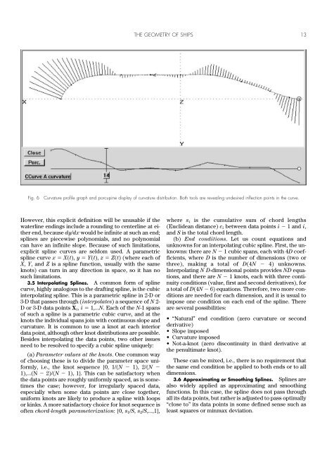
Fig. 6<br />
Curvature pr<strong>of</strong>ile graph and porcupine display <strong>of</strong> curvature distribution. Both tools are revealing undesired inflection points in the curve.<br />
However, this explicit definition will be unusable if the<br />
waterline endings include a rounding to centerline at either<br />
end, because dy/dx would be infinite at such an end;<br />
splines are piecewise polynomials, and no polynomial<br />
can have an infinite slope. Because <strong>of</strong> such limitations,<br />
explicit spline curves are seldom used. A parametric<br />
spline curve x X(t), y Y(t), z Z(t) (where each <strong>of</strong><br />
X, Y, and Z is a spline function, usually with the same<br />
knots) can turn in any direction in space, so it has no<br />
such limitations.<br />
3.5 Interpolating Splines. A common form <strong>of</strong> spline<br />
curve, highly analogous to the drafting spline, is the cubic<br />
interpolating spline. This is a parametric spline in 2-D or<br />
3-D that passes through (interpolates) a sequence <strong>of</strong> N 2-<br />
D or 3-D data points X i , i 1,...N. Each <strong>of</strong> the N-1 spans<br />
<strong>of</strong> such a spline is a parametric cubic curve, and at the<br />
knots the individual spans join with continuous slope and<br />
curvature. It is common to use a knot at each interior<br />
data point, although other knot distributions are possible.<br />
Besides interpolating the data points, two other issues<br />
need to be resolved to specify a cubic spline uniquely:<br />
(a) Parameter values at the knots. One common way<br />
<strong>of</strong> choosing these is to divide the parameter space uniformly,<br />
i.e., the knot sequence {0, 1/(N 1), 2/(N <br />
1),...(N 2)/(N 1), 1}. This can be satisfactory when<br />
the data points are roughly uniformly spaced, as is sometimes<br />
the case; however, for irregularly spaced data,<br />
especially when some data points are close together,<br />
uniform knots are likely to produce a spline with loops<br />
or kinks. A more satisfactory choice for knot sequence is<br />
<strong>of</strong>ten chord-length parameterization: {0, s 1 /S, s 2 /S,...,1},<br />
where s i is the cumulative sum <strong>of</strong> chord lengths<br />
(Euclidean distance) c i between data points i 1 and i,<br />
and S is the total chord length.<br />
(b) End conditions. Let us count equations and<br />
unknowns for an interpolating cubic spline. First, the unknowns:<br />
there are N 1 cubic spans, each with 4D coefficients,<br />
where D is the number <strong>of</strong> dimensions (two or<br />
three), making a total <strong>of</strong> D(4N 4) unknowns.<br />
Interpolating N D-dimensional points provides ND equations,<br />
and there are N 1 knots, each with three continuity<br />
conditions (value, first and second derivatives), for<br />
a total <strong>of</strong> D(4N 6) equations. <strong>The</strong>refore, two more conditions<br />
are needed for each dimension, and it is usual to<br />
impose one condition on each end <strong>of</strong> the spline. <strong>The</strong>re<br />
are several possibilities:<br />
• “Natural” end condition (zero curvature or second<br />
derivative)<br />
• Slope imposed<br />
• Curvature imposed<br />
• Not-a-knot (zero discontinuity in third derivative at<br />
the penultimate knot).<br />
<strong>The</strong>se can be mixed, i.e., there is no requirement that<br />
the same end condition be applied to both ends or to all<br />
dimensions.<br />
3.6 Approximating or Smoothing Splines. Splines are<br />
also widely applied as approximating and smoothing<br />
functions. In this case, the spline does not pass through<br />
all its data points, but rather is adjusted to pass optimally<br />
“close to” its data points in some defined sense such as<br />
least squares or minmax deviation.