

The Geometry of Ships

You also want an ePaper? Increase the reach of your titles
YUMPU automatically turns print PDFs into web optimized ePapers that Google loves.
24 THE PRINCIPLES OF NAVAL ARCHITECTURE SERIES<br />
incidentally by the elastic and/or plastic deformation accompanying<br />
stress and welding shrinkage that occurs<br />
during forced assembly <strong>of</strong> the product. In any case, introduction<br />
<strong>of</strong> in-plane strain is an expensive manufacturing<br />
process, and it is highly desirable to minimize the<br />
amount <strong>of</strong> it that is required. Also, it is very valuable to<br />
predict the flat blank outlines accurately so each plate,<br />
following forming, will fit “neat” to its neighbors, within<br />
weld-seam tolerances.<br />
<strong>The</strong>re exist traditional manual l<strong>of</strong>ting methods for<br />
plate expansion, some <strong>of</strong> which have been “computerized”<br />
as part <strong>of</strong> ship production CAD/CAM s<strong>of</strong>tware.<br />
Typically, these methods do not allow for the in-plane<br />
strain and, consequently, they produce results <strong>of</strong> limited<br />
utility for plates that are not nearly developable. A survey<br />
by Lamb (1995) showed that expansions <strong>of</strong> a test<br />
plate by four commercial s<strong>of</strong>tware systems yielded<br />
widely varying outlines.<br />
Letcher (1993) derived a second-order partial differential<br />
equation relating strain and Gaussian curvature<br />
distributions, and showed methods for numerical solution<br />
<strong>of</strong> this “strain equation” with appropriate boundary<br />
conditions. In production methods where plates are subjected<br />
to deliberate compound forming before assembly,<br />
this method has produced very accurate results, even for<br />
highly curved plates. When the forming is incidental to<br />
stress applied during assembly, results are less certain,<br />
as the details <strong>of</strong> the elastic stress field are not taken into<br />
account, and the process depends to some degree on the<br />
welding sequence (Fig. 20).<br />
Fig. 20 Plate expansion by numerical solution <strong>of</strong> the “strain equation.”<br />
(a) <strong>The</strong> plate is defined as a subsurface between snakes representing the<br />
seams. (b) <strong>The</strong> required strain distribution is indicated by contours, which<br />
are somewhat irregular on account <strong>of</strong> the discretization <strong>of</strong> the plate into<br />
triangular finite elements.<br />
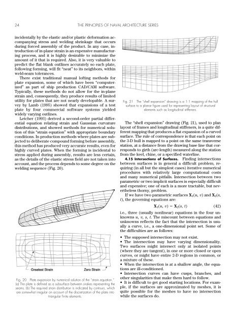
Fig. 21 <strong>The</strong> “shell expansion” drawing is a 1:1 mapping <strong>of</strong> the hull<br />
surface to a planar figure used for representing layout <strong>of</strong> structural<br />
elements such as longitudinal stiffeners.<br />
<strong>The</strong> “shell expansion” drawing (Fig. 21), used to plan<br />
layout <strong>of</strong> frames and longitudinal stiffeners, is a quite different<br />
mapping that produces a flat expansion <strong>of</strong> a curved<br />
surface. <strong>The</strong> rule <strong>of</strong> correspondence is that each point on<br />
the 3-D hull is mapped to a point on the same transverse<br />
station, at a distance from the drawing base line that corresponds<br />
to girth (arc-length) measured along the station<br />
from the keel, chine, or a specified waterline.<br />
4.15 Intersections <strong>of</strong> Surfaces. Finding intersections<br />
between surfaces is in general a difficult problem, requiring<br />
(in all but the simplest cases) iterative numerical<br />
procedures with relatively large computational costs<br />
and many numerical pitfalls. Intersection between two<br />
parametric or two implicit surfaces is especially difficult<br />
and expensive; one <strong>of</strong> each is a more tractable, but nevertheless<br />
thorny, problem.<br />
If we have two parametric surfaces X 1 (u, v) and X 2 (s,<br />
t), the governing equations are:<br />
X 1 (u, v) X 2 (s, t) (42)<br />
i.e., three (usually nonlinear) equations in the four unknowns<br />
u, v, s, t. <strong>The</strong> miscount between equations and<br />
unknowns reflects the fact that the intersection is usually<br />
a curve, i.e., a one-dimensional point set. Some <strong>of</strong><br />
the difficulties are as follows:<br />
• <strong>The</strong> supposed intersection may not exist.<br />
• <strong>The</strong> intersection may have varying dimensionality.<br />
Two surfaces might intersect only at isolated points<br />
(where they are tangent), in one or more closed or open<br />
curves, or might have entire 2-D regions in common, or<br />
a mixture <strong>of</strong> these.<br />
• When the intersection is at a shallow angle, the equations<br />
are ill-conditioned.<br />
• Intersection curves can have cusps, branches, and<br />
other singularities that make them hard to follow.<br />
• It is difficult to get good starting locations. For example,<br />
if the surfaces are approximated by meshes, it is<br />
quite possible for the meshes to have no intersection<br />
while the surfaces do.