

The Geometry of Ships

Create successful ePaper yourself
Turn your PDF publications into a flip-book with our unique Google optimized e-Paper software.
THE GEOMETRY OF SHIPS 21<br />
4.9 B-spline (Tensor-Product) Surface. A B-spline surface<br />
is defined in relation to a N u N v rectangular array<br />
(or net) <strong>of</strong> control points X ij by the surface equation:<br />
X(u,v) <br />
N u<br />
N v<br />
<br />
i1 j1<br />
X ij<br />
B i<br />
(u) B j<br />
(v)<br />
(39)<br />
where the B i (u) and B j (v) are B-spline basis functions <strong>of</strong><br />
specified order k u , k v for the u and v directions, respectively.<br />
<strong>The</strong> total amount <strong>of</strong> data required to define the<br />
surface is then:<br />
N u , N v number <strong>of</strong> control points for u and v directions<br />
k u , k v spline order for u and v directions<br />
U i , i 1, . . . N u k u , knotlist for u-direction<br />
V j , j 1, . . . N v k v , knotlist for v-direction<br />
X ij , i 1, . . . N u , j 1, . . . N v , control points.<br />
If the knots are uniformly spaced for both directions,<br />
the surface is a “uniform” B-spline (UBS) surface, otherwise<br />
it is “nonuniform” (NUBS). As in a B-spline curve,<br />
the B-spline products B i (u)B j (v) can be viewed as<br />
variable weights applied to the control points. <strong>The</strong> surface<br />
imitates the net in shape, but does it with a degree <strong>of</strong><br />
smoothness depending on the spline orders. Alternatively,<br />
you can envisage the surface patch as being attracted to<br />
the control points, or connected to them by springs.<br />
<strong>The</strong> following are useful properties <strong>of</strong> the B-spline<br />
surface, analogous to those <strong>of</strong> B-spline curves:<br />
• Corners: <strong>The</strong> four corners <strong>of</strong> the patch are at the four<br />
corner points <strong>of</strong> the net.<br />
• Edges: <strong>The</strong> four edges <strong>of</strong> the surface are the B-spline<br />
curves made from control points along the four edges <strong>of</strong><br />
the net.<br />
• Edge tangents: Slopes along edges are controlled by the<br />
two rows or columns <strong>of</strong> control points closest to the edge.<br />
• Straight sections: If k or more consecutive columns <strong>of</strong><br />
control points are copies <strong>of</strong> one another translated along<br />
an axis, a portion <strong>of</strong> the surface will be a general cylinder.<br />
• Local support: If N u k u or N v k v , the effect <strong>of</strong> any<br />
one control point is local, i.e., it only affects a limited<br />
portion (at most k u or k v spans) <strong>of</strong> the surface in the<br />
vicinity <strong>of</strong> the point.<br />
• Rigid body: <strong>The</strong> shape <strong>of</strong> the surface is invariant<br />
under rigid-body transformations <strong>of</strong> the net.<br />
• Affine: <strong>The</strong> surface scales affinely in response to<br />
affine scaling <strong>of</strong> the net.<br />
• Convex hull: <strong>The</strong> surface does not extend beyond the<br />
convex hull <strong>of</strong> the control points, i.e., the minimal closed<br />
convex polyhedron enclosing the control points.<br />
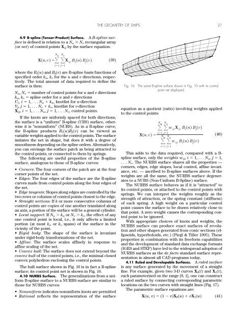
<strong>The</strong> hull surface shown in Fig. 10 is in fact a B-spline<br />
surface; its control point net is shown in Fig. 16.<br />
4.10 NURBS Surface. <strong>The</strong> generalizations from a uniform<br />
B-spline surface to a NURBS surface are similar to<br />
those for NURBS curves:<br />
• Nonuniform indicates nonuniform knots are permitted<br />
• Rational reflects the representation <strong>of</strong> the surface<br />
Fig. 16<br />
<strong>The</strong> same B-spline surface shown in Fig. 10 with its control<br />
point net displayed.<br />
equation as a quotient (ratio) involving weights applied<br />
to the control points:<br />
X(u,v) <br />
N u<br />
i1<br />
N v<br />
w ij<br />
X ij<br />
B i<br />
(u) B j<br />
(v)<br />
j1<br />
N u<br />
i1<br />
N v<br />
w ij<br />
B i<br />
(u) B j<br />
(v)<br />
j1<br />
(40)<br />
This adds to the data required, compared with a B-<br />
spline surface, only the weights w ij , i 1, . . . N u , j 1,<br />
. . . N v . <strong>The</strong> NURBS surface shares all the properties —<br />
corners, edges, edge slopes, local control, affine invariance,<br />
etc. — ascribed to B-spline surfaces above. If the<br />
weights are all the same, the NURBS surface degenerates<br />
to a NUBS (Non-Uniform B-Spline) surface.<br />
<strong>The</strong> NURBS surface behaves as if it is “attracted” to<br />
its control points, or attached to the control points with<br />
springs. We can interpret the weights roughly as the<br />
strength <strong>of</strong> attraction, or the spring constant (stiffness)<br />
<strong>of</strong> each spring. A high weight on a particular control<br />
point causes the surface to be drawn relatively close to<br />
that point. A zero weight causes the corresponding control<br />
point to be ignored.<br />
With appropriate choices <strong>of</strong> knots and weights, the<br />
NURBS surface can produce exact surfaces <strong>of</strong> revolution<br />
and other shapes generated from conic sections (ellipsoids,<br />
hyperboloids, etc.) (Piegl & Tiller 1995). <strong>The</strong>se<br />
properties in combination with its freeform capabilities<br />
and the development <strong>of</strong> standard data exchange formats<br />
(IGES and STEP) have led to the widespread adoption <strong>of</strong><br />
NURBS surfaces as the de facto standard surface representation<br />
in almost all CAD programs today.<br />
4.11 Ruled and Developable Surfaces. A ruled surface<br />
is any surface generated by the movement <strong>of</strong> a straight<br />
line. For example, given two 3-D curves X 0 (t) and X 1 (t),<br />
each parameterized on the range [0, 1], one can construct<br />
a ruled surface by connecting corresponding parametric<br />
locations on the two curves with straight lines (Fig. 17).<br />
<strong>The</strong> parametric surface equations are:<br />
X(u, v) (1 v)X 0 (u) vX 1 (u) (41)