The Geometry of Ships

THE GEOMETRY OF SHIPS 15
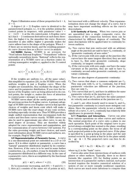
Figure 8 illustrates some of these properties for k 4,
N 6.
A degree-1 (k 2) B-spline curve is identical to the
parameterized polygon; i.e., it is the polyline joining the
control points in sequence, with parameter value t
(i 1)/(N 1) at the ith control point. A B-spline curve
x(t) has k 2 continuous derivatives at each knot; therefore,
the higher k is, the smoother the curve. However,
smoother is also stiffer; higher k generally makes the
curve adhere less to the shape of the polygon. When k
N there are no interior knots, and the resulting parametric
curve (known then as a Bezier curve) is analytic.
3.8 NURBS Curves. NURBS is an acronym for
“NonUniform Rational B-splines.” “Nonuniform” reflects
optionally nonuniform knots. “Rational” reflects the representation
of a NURBS curve as a fraction (ratio) involving
nonnegative weights w i applied to the N control
points:
N
i1
N
i1
x(t) w i
X i
B i
(t) w i
B i
(t)
(27)
If the weights are uniform (i.e., all the same value),
this simplifies to equation (26), so the NURBS curve with
uniform weights is just a B-spline curve. When the
weights are nonuniform, they modulate the shape of the
curve and its parameter distribution. If you view the behavior
of the B-spline curve as being attracted to its control
points, the weight w i makes the force of attraction
to control point i stronger or weaker.
NURBS curves share all the useful properties cited in
the previous section for B-spline curves. A primary advantage
of NURBS curves over B-spline curves is that specific
choices of weights and knots exist which will make a
NURBS curve take the exact shape of any conic section,
including especially circular arcs. Thus NURBS provides a
single unified representation that encompasses both the
conics and free-form curves exactly. NURBS curves can
also be used to approximate any other curve, to any desired
degree of accuracy. They are therefore widely
adopted for curve representation and manipulation, and
for communication of curves between CAD systems. For
the rules governing weight and knot choices, and much
more information about NURBS curves and surfaces, see,
for example, Piegl & Tiller (1995).
3.9 Reparameterization of Parametric Curves. A curve
is a one-dimensional point set embedded in a 2-D or 3-D
space. If it is either explicit or parametric, a curve has a
“natural” parameter distribution implied by its construction.
However, if the curve is to be used in some further
construction, e.g., of a surface, it may be desirable to have
its parameter distributed in a different way. In the case of
a parametric curve, this is accomplished by the functional
composition:
y(t) x(t), where t f(t). (28)
If f is monotonic increasing, and f(0) 0 and f(1)
1, then y(t) consists of the same set of points as x(t),
but traversed with a different velocity. Thus reparameterization
does not change the shape of a curve, but it
may have important modeling effects on the curve’s
descendants.
3.10 Continuity of Curves. When two curves join or
are assembled into a single composite curve, the
smoothness of the connection between them can be
characterized by different degrees of continuity. The
same descriptions will be applied later to continuity between
surfaces.
G 0 : Two curves that join end-to-end with an arbitrary
angle at the junction are said to have G 0 continuity, or
“geometric continuity of zero order.”
G 1 : If the curves join with zero angle at the junction (the
curves have the same tangent direction) they are said
to have G 1 , first order geometric continuity, slope
continuity, or tangent continuity.
G 2 : If the curves join with zero angle, and have the same
curvature at the junction, they are said to have G 2
continuity, second order geometric continuity, or curvature
continuity.
There are also degrees of parametric continuity:
C 0 : Two curves that share a common endpoint are C 0 .
They may join with G 1 or G 2 continuity, but if their
parametric velocities are different at the junction,
they are only C 0 .
C 1 : Two curves that are G 1 and have in addition the same
parametric velocity at the junction are C 1 .
C 2 : Two curves that are G 2 and have the same parametric
velocity and acceleration at the junction are C 2 .
C 1 and C 2 are often loosely used to mean G 1 and G 2 ,
but parametric continuity is a much more stringent condition.
Since the parametric velocity is not a visible attribute
of a curve, C 1 or C 2 continuity has relatively little
significance in geometric design.
3.11 Projections and Intersections. Curves can arise
from various operations on other curves and surfaces.
The normal projection of a curve onto a plane is one
such operation. Each point of the original curve is projected
along a straight line normal to the plane, resulting
in a corresponding point on the plane; the locus of all
such projected points is the projected curve. If the plane
is specified by a point p lying in the plane and the unit
normal vector û, the points x that lie in the plane satisfy
(x p) û 0. The projected curve can then be described
by
x(t) x 0 (t) û[(x 0 (t) p) û] (29)
where x 0 (t) is the “basis” curve.
Curves also arise from intersections of surfaces with
planes or other surfaces. Typically, there is no direct
formula like equation (29) for finding points on an
intersection of a parametric surface; instead, each point
located requires the iterative numerical solution of a
system of one or more (usually nonlinear) equations.
Such curves are much more laborious to compute than