PDF (1016 kB)

More documents

Recommendations

Info

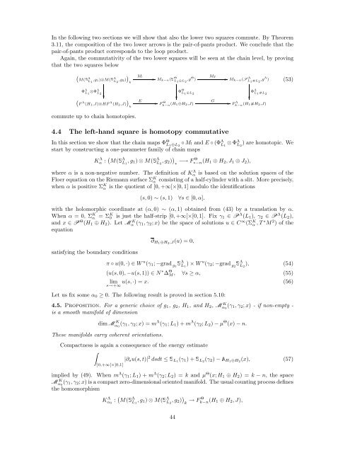
In the following two sections we will show that also the lower two squares commute. By Theorem 3.11, the composition of the two lower arrows is the pair-of-pants product. We conclude that the pair-of-pants product corresponds to the loop product. Again, the commutativity of the two lower squares will be seen at the chain level, by proving that the two squares below � � M(ËΛ L ,g1)⊗M(ËΛ 1 L ,g2) 2 k Φ Λ L 1 ⊗Φ Λ L 2 � F Λ (H1,J)⊗HF Λ (H2,J) commute up to chain homotopies. �� k M! E �� Mk−n(ËΘ L 1 ⊕L 2 ,g Θ ) �� Φ �� Θ L1⊕L2 F Θ k−n (H1⊕H2,J) 4.4 The left-hand square is homotopy commutative MΓ G �� Mk−n(S Λ L 1 #L 2 ,g Λ ) �� Φ �� Λ L1 #L2 F Λ k−n (H1#H2,J) In this section we show that the chain maps ΦΘ L1⊕L2 ◦ M! and E ◦ (ΦΛ L1 ⊗ ΦΛ ) are homotopic. We L2 start by constructing a one-parameter family of chain maps K Λ α : � M(ËΛ , g1) ⊗ M(ËΛ , g2) L1 L2 � ∗ −→ F Θ ∗−n (H1 ⊕ H2, J1 ⊕ J2), where α is a non-negative number. The definition of KΛ α is based on the solution spaces of the consisting of a half-cylinder with a slit. More precisely, Floer equation on the Riemann surface ΣK α when α is positive ΣK α is the quotient of [0, +∞[×[0, 1] modulo the identifications (s, 0) ∼ (s, 1) ∀s ∈ [0, α]. with the holomorphic coordinate at (α, 0) ∼ (α, 1) obtained from (43) by a translation by α. When α = 0, Σ K α = Σ K 0 is just the half-strip [0, +∞[×[0, 1]. Fix γ1 ∈ P Λ (L1), γ2 ∈ P Λ (L2), and x ∈ P Θ (H1 ⊕ H2). Let M K α (γ1, γ2; x) be the space of solutions u ∈ C ∞ (Σ K α , T ∗ M 2 ) of the equation satisfying the boundary conditions ∂H1⊕H2,J(u) = 0, (53) π ◦ u(0, ·) ∈ W u (γ1; −grad g1ËΛ L1 ) × W u (γ2; −grad g2ËΛ L2 ), (54) (u(s, 0), −u(s, 1)) ∈ N ∗ ∆ Θ M , ∀s ≥ α, (55) lim u(s, ·) = x. s→+∞ (56) Let us fix some α0 ≥ 0. The following result is proved in section 5.10: 4.5. Proposition. For a generic choice of g1, g2, H1, and H2, M K α0 (γ1, γ2; x) - if non-empty - is a smooth manifold of dimension dimM K α0 (γ1, γ2; x) = m Λ (γ1; L1) + m Λ (γ2; L2) − µ Θ (x) − n. These manifolds carry coherent orientations. Compactness is again a consequence of the energy estimate � |∂su(s, t)| 2 dsdt ≤ËL1(γ1) +ËL2(γ2) −�H1⊕H2(x), (57) ]0,+∞[×]0,1[ implied by (49). When m Λ (γ1; L1) + m Λ (γ2; L2) = k and µ Θ (x; H1 ⊕ H2) = k − n, the space M K α0 (γ1, γ2; x) is a compact zero-dimensional oriented manifold. The usual counting process defines the homomorphism K Λ α0 : � M(ËΛ L1 , g1) ⊗ M(ËΛ L2 , g2) � k → F Θ k−n (H1 ⊕ H2, J), 44
and a standard gluing argument shows that KΛ is a chain map. α0 Now assume α0 > 0. By standard compactness and gluing arguments, the family of solutions M K α for α varying in the interval [α0, +∞[ allows to define a chain homotopy between KΛ α0 and the composition E ◦ (ΦΛ L1 ⊗ ΦΛL2 ). Similarly, a compactness and cobordism argument on the Morse side shows that KΛ 0 is chain homotopic to the composition ΦΘ L1⊕L2 ◦ M!. See Figure 5. α Θ E ◦ (Φ Λ L1 ⊗ ΦΛ L2 ) ≃ KΛ α Θ ! ≃ KΛ 0 ≃ ΦΘ ◦ M! L1⊕L2 Figure 5: The homotopy through K Λ α and K Λ 0 . There remains to prove that KΛ α0 is homotopic to KΛ 0 . Constructing a homotopy between these chain maps by using the spaces of solutions M K α for α ∈ [0, α0] presents analytical difficulties: if we are given a solution u of the limiting problem M K 0 , the existence of a (unique) one-parameter family of solutions ”converging” to u is problematic, because we do not expect u to be C0 close to the one-parameter family of solutions, due to the jump in the boundary conditions. Therefore, we use a detour, starting from the following algebraic observation. If two chain maps ϕ, ψ : C → C ′ are homotopic, so are their tensor products ϕ ⊗ψ and ψ ⊗ϕ. The converse is obviously not true, as the example of ϕ = 0 and ψ non-contractible shows. However, it becomes true under suitable conditions on ϕ and ψ. Denote by (�, 0) the graded group which vanishes at every degree, except for degree zero where it coincides with�. We see (�, 0) as a chain complex with the trivial boundary operator. We have the following: 4.6. Lemma. Let (C, ∂) and (C ′ , ∂) be chain complexes, bounded from below. Let ϕ, ψ : C → C ′ be chain maps. Assume that there is an element ǫ ∈ C0 with ∂ǫ = 0 and a chain map δ : C ′ → (�, 0) such that δ(ϕ(ǫ)) = δ(ψ(ǫ)) = 1. If ϕ ⊗ ψ is homotopic to ψ ⊗ ϕ then ϕ is homotopic to ψ Proof. Let π be the chain map π : C ′ ⊗ C ′ → C ′ ⊗ (�, 0) ∼ = C ′ , π = id ⊗ δ. Let H : C ⊗ C → C ′ ⊗ C ′ be a chain homotopy between ϕ ⊗ ψ and ψ ⊗ ϕ, that is If we define the homomorphism h : C → C ′ by we have ϕ ⊗ ψ − ψ ⊗ ϕ = ∂H + H∂. h(a) := π ◦ H(a ⊗ ǫ), ∀a ∈ C, ∂h(a) + h∂a = ∂π(H(a ⊗ ǫ)) + π(H∂(a ⊗ ǫ)) = π(∂H(a ⊗ ǫ) + H∂(a ⊗ ǫ)) = π(ϕ(a) ⊗ ψ(ǫ) − ψ(a) ⊗ ϕ(ǫ)) = ϕ(a) ⊗ δ(ψ(ǫ)) − ψ(a) ⊗ δ(ϕ(ǫ)) = ϕ(a) − ψ(a). Hence h is the required chain homotopy. 45
Page 1: Å�ÜÈÐ�Ò�ÁÒ×Ø�ØÙ
Page 4 and 5: 5.8 Non-local boundary conditions .
Page 6 and 7: M into Λ(M) as the space of consta
Page 8 and 9: and converging to Hamiltonian orbit
Page 10 and 11: 1.2 The Chas-Sullivan loop product
Page 12 and 13: 1.1. Remark. The loop product was d
Page 14 and 15: 2.2 Functoriality Let (M1, g1) and
Page 16 and 17: The orbits of −grad(f1 ⊕f2) are
Page 18 and 19: this intersection is a finite set o
Page 20 and 21: (L0) Ω every solution γ ∈ P
Page 22 and 23: transverse to the stable manifold o
Page 24 and 25: 2.7. Proposition. The homomorphism
Page 26 and 27: A submanifold L ⊂ T ∗ M is call
Page 28 and 29: The L 2 -negative gradient equation
Page 30 and 31: The Riemann surface Σ Ω Υ s = 0
Page 32 and 33: In the periodic case, we consider H
Page 34 and 35: 3.6. Definition. The Maslov index
Page 36 and 37: The Riemann surface ΣG is obtained
Page 38 and 39: 3.12. Proposition. For a generic ch
Page 40 and 41: The following compactness statement
Page 42 and 43: 4.2. Proposition. For a generic cho
Page 44 and 45: A standard gluing argument shows th
Page 48 and 49: We shall apply the above lemma to t
Page 50 and 51: Since the inclusion c : M ֒→ Λ
Page 52 and 53: 4.5 The right-hand square is homoto
Page 54 and 55: commute. Our first aim in this sect
Page 56 and 57: Moreover, �Dαn(βnvn)�0,p;Ê
Page 58 and 59: We identify the product T ∗Ên ×
Page 60 and 61: Up to multiplying u by U, we can re
Page 62 and 63: The symbol C∞ S ,c indicates boun
Page 64 and 65: 5.11. Theorem. (Cauchy-Riemann oper
Page 66 and 67: 5.15. Lemma. Let p > 1 and α ∈Ê
Page 68 and 69: Proof. By Proposition 5.14 the oper
Page 70 and 71: Then ind∂A = ind∂A1 + ind∂A1.
Page 72 and 73: (V0, . . . , Vk), by V ′ the (k
Page 74 and 75: is bounded and Fredholm of index in
Page 76 and 77: so the transversality hypotheses of
Page 78 and 79: 5.9 Coherent orientations As notice
Page 80 and 81: compact subsets of Σ Ω Υ , for
Page 82 and 83: where Ã(z) = CA(z)C ⊕ A(z), C de
Page 84 and 85: By the additivity property of the M
Page 86 and 87: The space M Υ GE . Let x1 ∈ P(H1
Page 88 and 89: The space M Θ Φ . Let γ ∈ PΘ
Page 90 and 91: The embedding Q ֒→ÊN induces an
Page 92 and 93: Given periodic orbits x1 ∈ P(H1),
Page 94 and 95: Since u and ∂u are integrable ove
Page 96 and 97:
with non-local boundary conditions
Page 98 and 99:
to ũ0 uniformly on Σ, we may loca
Page 100 and 101:
we see that associating ũ to u pro
Page 102 and 103:
The energy of a solution u ∈ M K
Page 104 and 105:
Since we have applied a conformal r
Page 106 and 107:
6.9. Lemma. There exists a positive
Page 108 and 109:
[ChS04] M. Chas and D. Sullivan, Cl
show all

PDF (1016 kB)

Create successful ePaper yourself

Delete template?

Save as template?