Particle Physics Booklet - Particle Data Group - Lawrence Berkeley ...

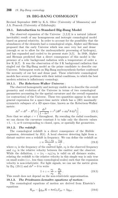
208 19. Big-Bang cosmology
19. BIG-BANG COSMOLOGY
Revised September 2009 by K.A. Olive (University of Minnesota) and
J.A. Peacock (University of Edinburgh).
19.1. Introduction to Standard Big-Bang Model
The observed expansion of the Universe [1,2,3] is a natural (almost
inevitable) result of any homogeneous and isotropic cosmological model
based on general relativity. In order to account for the possibility that the
abundances of the elements had a cosmological origin, Alpher and Herman
proposed that the early Universe which was once very hot and dense
(enough so as to allow for the nucleosynthetic processing of hydrogen),
and has expanded and cooled to its present state [4,5]. In 1948, Alpher
and Herman predicted that a direct consequence of this model is the
presence of a relic background radiation with a temperature of order a
few K [6,7]. It was the observation of the 3 K background radiation that
singled out the Big-Bang model as the prime candidate to describe our
Universe. Subsequent work on Big-Bang nucleosynthesis further confirmed
the necessity of our hot and dense past. These relativistic cosmological
models face severe problems with their initial conditions, to which the best
modern solution is inflationary cosmology.
19.1.1. The Robertson-Walker Universe :
The observed homogeneity and isotropy enable us to describe the overall
geometry and evolution of the Universe in terms of two cosmological
parameters accounting for the spatial curvature and the overall expansion
(or contraction) of the Universe. These two quantities appear in the most
general expression for a space-time metric which has a (3D) maximally
symmetric subspace of a 4D space-time, known as the Robertson-Walker
metric:
ds 2 = dt 2 − R 2 �
dr2 (t)
1 − kr2 + r2 (dθ 2 +sin 2 θdφ 2 �
) . (19.1)
Note that we adopt c = 1 throughout. By rescaling the radial coordinate,
we can choose the curvature constant k to take only the discrete values
+1, −1, or 0 corresponding to closed, open, or spatially flat geometries.
19.1.2. The redshift :
The cosmological redshift is a direct consequence of the Hubble
expansion, determined by R(t). A local observer detecting light from a
distant emitter sees a redshift in frequency. We can define the redshift as
z ≡ ν1 − ν2
�
ν2
v12
, (19.3)
c
where ν1 is the frequency of the emitted light, ν2 is the observed frequency
and v12 is the relative velocity between the emitter and the observer.
While the definition, z =(ν1− ν2)/ν2 is valid on all distance scales,
relating the redshift to the relative velocity in this simple way is only true
on small scales (i.e., less than cosmological scales) such that the expansion
velocity is non-relativistic. For light signals, we can use the metric given
by Eq. (19.1) and ds2 =0towrite
1+z = ν1
=
ν2
R2
. (19.5)
R1
This result does not depend on the non-relativistic approximation.
19.1.3. The Friedmann-Lemaître equations of motion :
The cosmological equations of motion are derived from Einstein’s
equations
Rμν − 1 2 gμνR =8πGNTμν +Λgμν . (19.6)