Particle Physics Booklet - Particle Data Group - Lawrence Berkeley ...

33. STATISTICS
33. Statistics 271
Revised September 2009 by G. Cowan (RHUL).
There are two main approaches to statistical inference, which we
may call frequentist and Bayesian. In frequentist statistics, probability is
interpreted as the frequency of the outcome of a repeatable experiment.
The most important tools in this framework are parameter estimation,
covered in Section 33.1, and statistical tests, discussed in Section 33.2.
Frequentist confidence intervals, which are constructed so as to cover
the true value of a parameter with a specified probability, are treated in
Section 33.3.2. Note that in frequentist statistics one does not define a
probability for a hypothesis or for a parameter.
In Bayesian statistics, the interpretation of probability is more general
and includes degree of belief (called subjective probability). One can then
speak of a probability density function (p.d.f.) for a parameter, which
expresses one’s state of knowledge about where its true value lies. Using
Bayes’ theorem Eq. (32.4), the prior degree of belief is updated by the
data from the experiment. Bayesian methods for interval estimation are
discussed in Sections 33.3.1 and 33.3.2.6
Following common usage in physics, the word “error” is often used in
this chapter to mean “uncertainty.” More specifically it can indicate the
size of an interval as in “the standard error” or “error propagation,” where
the term refers to the standard deviation of an estimator.
33.1. Parameter estimation
Here we review the frequentist approach to point estimationof
parameters. An estimator � θ (written with a hat) is a function of the data
whose value, the estimate, is intended as a meaningful guess for the value
of the parameter θ.
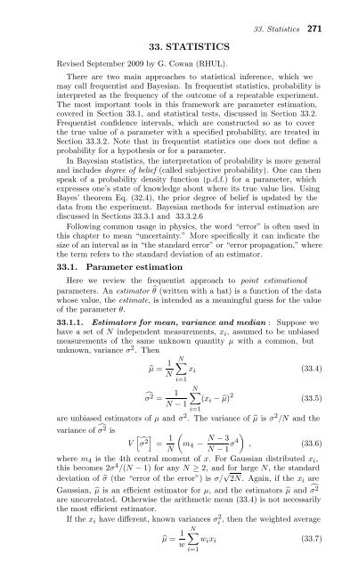
33.1.1. Estimators for mean, variance and median : Suppose we
have a set of N independent measurements, xi, assumed to be unbiased
measurements of the same unknown quantity μ with a common, but
unknown, variance σ2 .Then
�μ = 1
N�
xi
(33.4)
N
i=1
�σ 2 = 1
N�
(xi − �μ)
N − 1
i=1
2
(33.5)
are unbiased estimators of μ and σ2 . The variance of �μ is σ2 /N and the
variance of � σ2 is
� �
V �σ 2 = 1
�
N − 3
m4 −
N N − 1 σ4
�
, (33.6)
where m4 is the 4th central moment of x. For Gaussian distributed xi,
this becomes 2σ4 /(N − 1) for any N ≥ 2, and for large N, the standard
deviation of �σ (the “error of the error”) is σ/ √ 2N. Again, if the xi are
Gaussian, �μ is an efficient estimator for μ, and the estimators �μ and � σ2 are uncorrelated. Otherwise the arithmetic mean (33.4) is not necessarily
the most efficient estimator.
If the xi have different, known variances σ2 i , then the weighted average
�μ = 1
N�
wixi
(33.7)
w
i=1