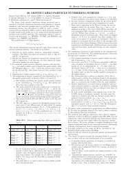
Particle Physics Booklet - Particle Data Group - Lawrence Berkeley ...

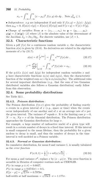
268 32. Probability
� ∞ � ∞
σx = (x − μx)
−∞ −∞
2 f(x, y) dx dy . Note ρ 2 xy ≤ 1.
• Independence: x,y are independent if and only if f(x, y) =f1(x) · f2(y);
then ρxy =0,E[u(x) v(y)] = E[u(x)] E[v(y)] and V [x+y] =V [x]+V [y].
• Change of variables: From x = (x1,...,xn) to y = (y1,...,yn):
g(y) =f (x(y)) ·|J| where |J| is the absolute value of the determinant of
the Jacobian Jij = ∂xi/∂yj. For discrete variables, use |J| =1.
32.3. Characteristic functions
Given a pdf f(x) for a continuous random variable x, the characteristic
function φ(u) is given by (31.6). Its derivatives are related to the algebraic
moments of x by (31.7).
�
φ(u) =E e iux�
� ∞
= e
−∞
iux f(x) dx . (32.17)
i −n dnφ dun � �
� ∞
�
� = x
u=0 −∞
n f(x) dx = αn . (32.18)
If the p.d.f.s f1(x) andf2(y) for independent random variables x and
y have characteristic functions φ1(u) andφ2(u), then the characteristic
function of the weighted sum ax+ by is φ1(au)φ2(bu). The additional rules
for several important distributions (e.g., that the sum of two Gaussian
distributed variables also follows a Gaussian distribution) easily follow
from this observation.
32.4. Some probability distributions
See Table 32.1.
32.4.2. Poisson distribution :
The Poisson distribution f(n; ν) gives the probability of finding exactly
n events in a given interval of x (e.g., space or time) when the events
occur independently of one another and of x at an average rate of ν per
the given interval. The variance σ2 equals ν. It is the limiting case p → 0,
N →∞, Np = ν of the binomial distribution. The Poisson distribution
approaches the Gaussian distribution for large ν.
For example, a large number of radioactive nuclei of a given type will
result in a certain number of decays in a fixed time interval. If this interval
is small compared to the mean lifetime, then the probability for a given
nucleus to decay is small, and thus the number of decays in the time
interval is well modeled as a Poisson variable.
32.4.3. Normal or Gaussian distribution :
Its cumulative distribution, for mean 0 and variance 1, is usually tabulated
as the error function
F (x;0, 1) = 1
2
�
1+erf(x/ √ �
2) . (32.24)
For mean μ and variance σ 2 , replace x by (x − μ)/σ. The error function is
acessible in libraries of computer routines such as CERNLIB.
P (x in range μ ± σ) = 0.6827,
P (x in range μ ± 0.6745σ) = 0.5,
E[|x − μ|] = � 2/πσ =0.7979σ,
half-width at half maximum = √ 2ln2· σ =1.177σ.