Particle Physics Booklet - Particle Data Group - Lawrence Berkeley ...

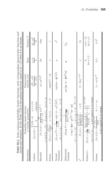
Table 32.1. Some common probability density functions, with corresponding characteristic functions and
means and variances. In the Table, Γ(k) is the gamma function, equal to (k − 1)! when k is an integer.
Probability density function Characteristic
Distribution f (variable; parameters) function φ(u) Mean Variance σ2 �
1/(b − a) a ≤ x ≤ b
e
Uniform f(x; a, b) =
0 otherwise
ibu − eiau a + b
(b − a)
(b − a)iu
2
2
12
N!
Binomial f(r; N,p) =
r!(N − r)! prqN−r (q + peiu ) N Np Npq
r =0, 1, 2,...,N ; 0 ≤ p ≤ 1; q =1− p
; n =0, 1, 2,... ; ν>0 exp[ν(e iu − 1)] ν ν
Poisson f(n; ν) = νne−ν n!
f(x; μ, σ2 )= 1
σ √ 2π exp(−(x − μ)2 /2σ2 ) exp(iμu − 1 2σ2 u2 ) μ σ2 −∞